
Characteristics analysis of quantity and spatial structure of standing live and dead trees in Tilia amurensis secondary forest on the west slope of Zhangguangcailing, northeastern China
-
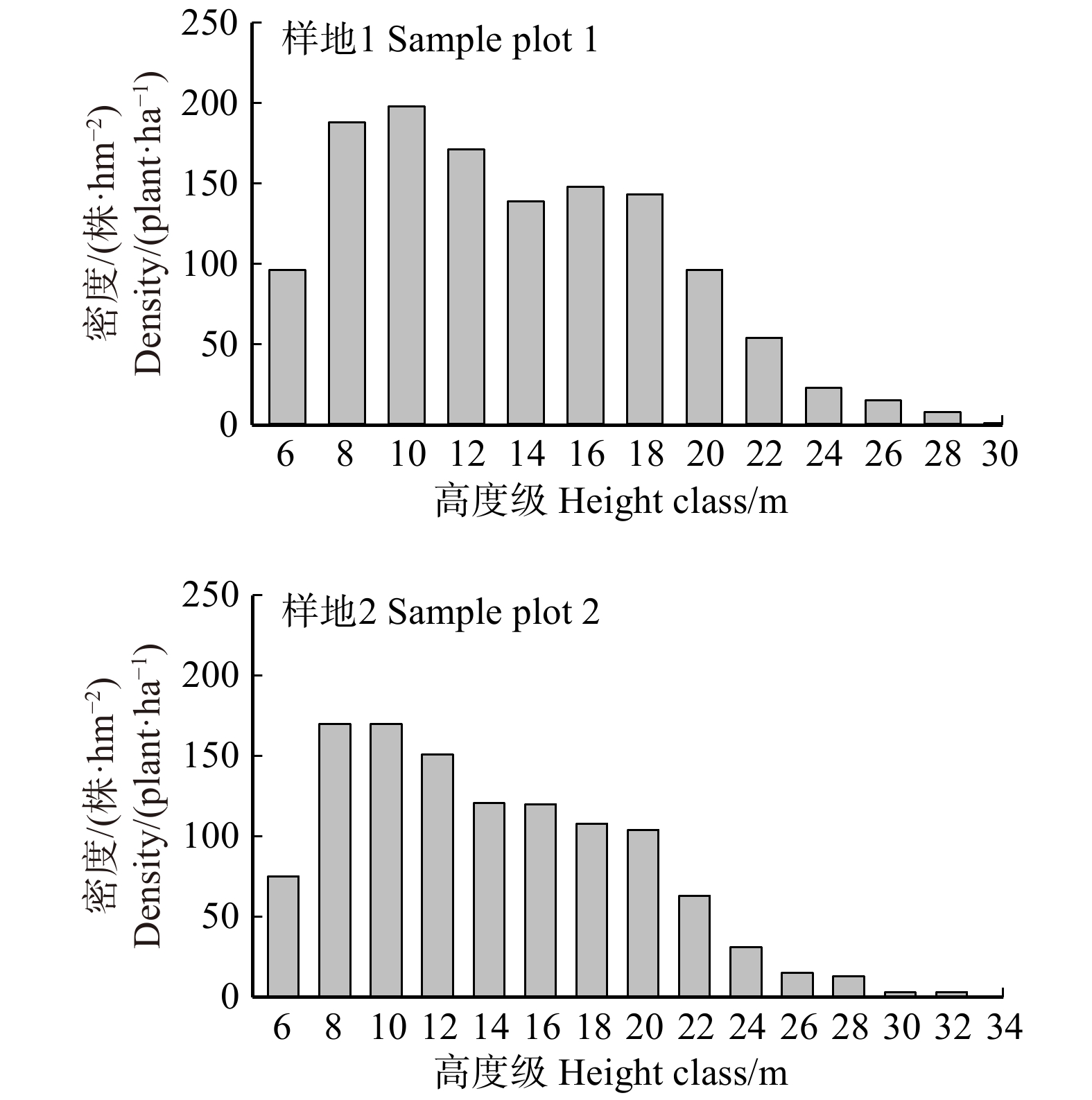
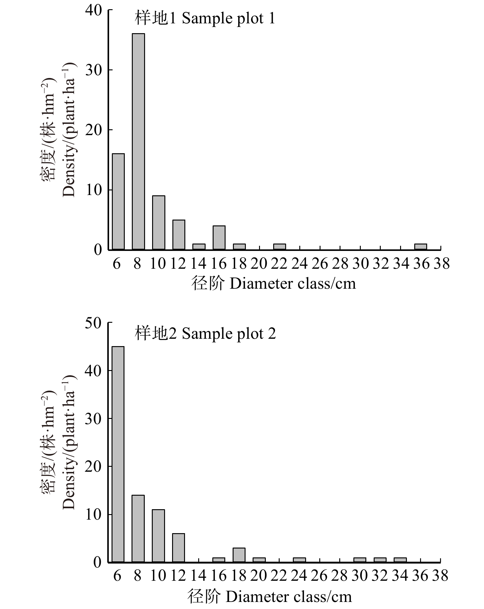
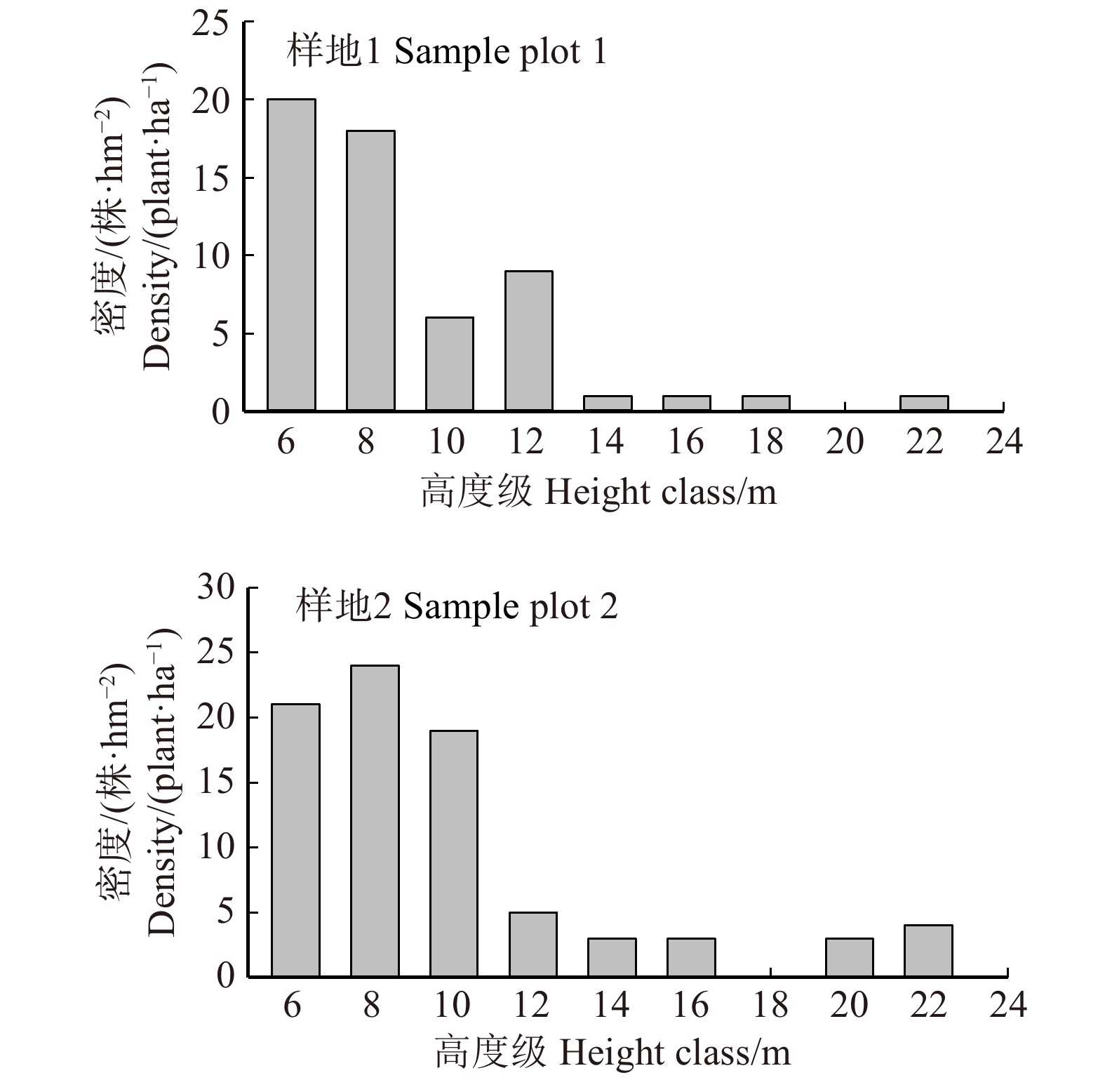
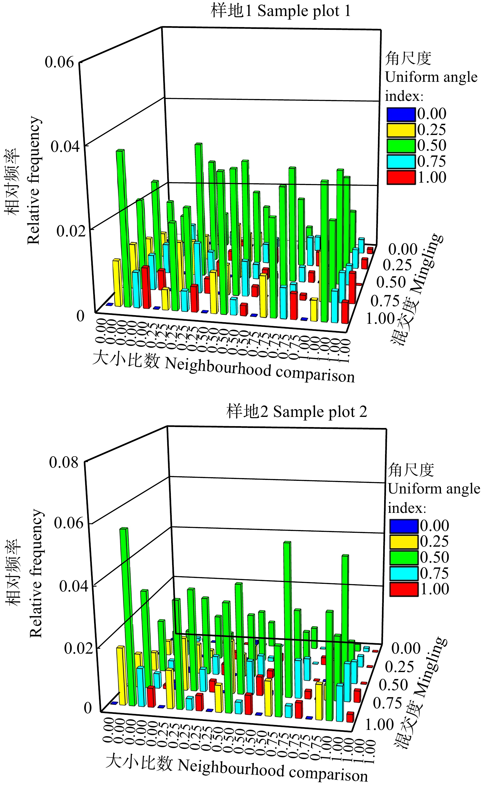
摘要:目的通过分析两种干扰模式(未择伐、择伐)下紫椴次生林中枯立木和活立木的数量及空间结构特征,探究林分生长状态、演替过程以及枯立木形成的主要原因,为紫椴次生林的生长、保护以及经营提供依据。方法分析活立木、枯立木物种组成、径级结构、高度级结构及空间结构。结果(1)在择伐林分中,紫椴和色木槭以及其他活立木占优势地位的树种在枯立木中也同样占优势地位,而未择伐林分中,紫椴在活立木和枯立木中占优势,但色木槭只在活立木中占优势,枯立木中并不多见。(2)两个林分中小径阶的活立木和枯立木均占优势,径阶结构均大致呈倒J型。两个林分活立木高度级结构大致呈左偏山峰状,而枯立木大致呈倒J型,小个体枯立木所占比例较大,因此可以分析出两个林分枯立木形成主要的原因是林木间竞争。(3)由空间结构参数三元分析可知,两个林分中呈随机分布、高度混交且占优势的活立木较多。而大多数枯立木处于随机分布、劣势状态,且周围林木均为其他树种或仅有1株为同树种。(4)通过枯立木结构参数四元分布可知,两个林分枯立木总体呈现随机分布,具有很强的种间混交,且大小分化很明显。四元分布能反映出该状态下的枯立木周围存在3 ~ 4株活立木。【结论】 以上信息进一步说明林木种间竞争是该种林分枯立木形成的主要原因。该研究分析了2种紫椴次生林活立木及枯立木空间结构及数量特征,不仅可以探究该类型次生林枯立木形成的主要原因,也为其保护和经营提供了理论依据。Abstract:ObjectiveThe aim of this study was to provide a basis for the growth, protection and management of Tilia amurensis secondary forest by analyzing the quantity and spatial structure characteristics of standing live and dead trees and exploring the growth state, succession process and the main causes of standing dead trees under two disturbance modes (non-cutting and selective cutting).MethodThe research was conducted by analyzing the species composition, diameter structure, height structure and spatial structure of standing live and dead trees.Result(1) Tilia amurensis, Acer mono, as well as other dominant tree species in living trees also had a dominant position in dead trees in selective cutting stand, while only Tilia amurensis was dominate among the living trees and standing dead trees in non-cutting stand, but Acer mono was only dominate in the living trees, and it was rare in dead standing trees. (2) The standing live and dead trees of the small diameter were dominant in all two stands, and the diameter distribution was roughly inverted J type. The height class distribution of living trees was roughly left-skewed distribution in two stands, while the standing dead trees were inverted J type, meanwhile, the small standing dead trees accounted for a large proportion. Therefore, it could be analyzed that the main reason for the formation of dead trees in the two stands was the competition among trees. (3) The trivariate distribution of spatial structure parameters had shown that there were more dominant living trees, which were randomly distributed, highly mixed and dominant in two stands. Whereas, most of the standing dead trees were randomly distributed, in disadvantaged state, and the surrounding trees were all other tree species or only one was the same tree species. (4) The quadrivariate distribution of spatial structure parameters showed that the standing dead trees of the two stands were randomly distributed in general with good mixture of species and obvious size differentiation. There were three or four standing live trees around one standing dead trees in that state.ConclusionIt further indicates that inter-species competition is the main reason for the formation of standing dead trees. This study analyzed the spatial structure and quantitative characteristics of standing live and dead trees in the secondary forest of Tilia amurensis. Therefore it is not only exploring the formation of dead standing trees in the secondary forest, but also provides a theoretical basis for its protection and management.
-
中国木结构古建筑是人类文明长河中最悠久持续的传统建筑之一,其体系的完备和规范无与伦比,堪称中华文化瑰宝中的璀璨明珠[1]。木柱是木结构古建筑的关键承重构件之一,支撑着建筑顶部的全部重量。古建筑木柱根据其与墙体间的位置关系,可分为露明柱、半露明柱和墙内暗柱3类[2]。其中,墙内暗柱是指完全被墙体包裹的木柱,因其根部处于易潮湿和缺乏通风的环境,易产生腐朽及由严重腐朽导致的材料缺失等缺陷。这些缺陷会使木柱丧失原有的承重能力,给整个古建筑的安全带来隐患。
为了检测古建筑木柱内部以及被墙体遮挡处的缺陷,往往需要采用无损检测技术,这类非破坏式检测可在尽量保持材料和结构完整的前提下,利用现代物理手段和仪器对其缺陷情况以及物理力学性能进行检测与分析[3−4]。根据T/CECS714—2020《古建筑木结构检测标准》[5]和DB11/T1190.1—2015《古建筑结构安全性鉴定技术规范第一部分》[6],目前用于检测古建筑木柱缺陷的方法主要有微钻阻力法和应力波法等。陈勇平等[7]通过分析微钻阻力曲线的轮廓和走势,实现了对瓜棱柱露明柱内部结构的精确探测,从而推断出早期和后期瓜棱柱维修的差异。段新芳等[8]采用应力波测定仪FAKOPP对塔尔寺大金瓦殿部分木构件中的木柱进行了检测,结果表明应力波技术可以判断和测量木构件内部的缺陷情况和力学强度。张典等[2]、于永柱等[9]对故宫养心殿墙体木柱(半露明柱和墙内暗柱)缺陷状况进行了无损检测研究,对半露明柱的检查充分利用了木柱外露表面提供的仪器操作空间,而墙内暗柱利用透风墙体的通风口拆除部分砖块形成的拆口,作为仪器操作空间进行检查,并利用有限元进行了安全性分析。Kandemir-Yucel等[10]利用超声波速测量技术与其他技术结合对土耳其清真寺中的木结构进行无损检测,评估包括木柱在内的结构木构件的保存状态、潮湿情况与修复情况。
到目前为止,古建筑木柱无损检查研究和应用多针对的是露明柱和半露明柱,而对墙内暗柱缺陷状况检测相对很少,且往往需要利用墙内暗柱透风口并拆除部分砖块形成的拆口进行检测。这种墙内暗柱检查方式在一定程度上会破坏古建筑原有结构与形貌,且由于仪器无法全面铺开,存在检测死角,检测效果并不理想。因此,亟需一种不破坏古建筑结构的墙内暗柱无损检查方法。
红外热成像技术利用物体会按照温度辐射不同波长电磁波的原理,将检测物体发出的红外辐射转换为可视化温度场,实现对物体的缺陷测量[11]。有研究者将红外热成像技术应用到墙壁外保温层的热工缺陷、表面开裂和墙面间空鼓等的检测中。Grinzato等[12]通过热像仪记录温度的空间分布与时间演变过程,基于最合适的局部热参数对数据进行处理,以检测出墙体的缺陷分布,但无法检测具有较低热信号特征的缺陷。Tavukçuoğlu等[13]将红外热成像技术与超声波相结合,有效地检测了历史砌体的裂缝,并区分裂缝深度,但需要对区域进行连续热监测,以升温速率判断深度。Afshani等[14]基于被动热成像检测损伤的混凝土结构中的缺陷,解释了由于传导、对流和辐射机制引起的混凝土管片、隧道空气和空隙内部空气中的热量传递,并分析了空洞类型、温差和空洞深度对检测精度的影响。Martínez等 [15]利用被动红外热成像技术评估西班牙马德里木质屋顶建筑的缺陷情况,证明该技术可以检测热变化的缺陷,但环境因素与检测时间会影响热检测的效果,且没有进行主动热成像的缺陷检测研究。
本研究团队针对古建筑墙内暗柱缺陷状况检测困难的问题,基于红外热成像无损检测技术开展了相关研究。首先,从理论上分析墙体与木柱传热机理,以及缺陷参数对热传导的影响;然后,建立试验模型,进行墙内暗柱材料缺失红外检查试验,采集红外图像;最后,通过分析获得的红外热图,探讨墙内暗柱缺陷大小与墙体表面温度分布之间的关系。以期为基于红外热成像的墙内暗柱缺陷状况的材料缺失无损检测方法的建立,奠定部分前期基础。
1. 热成像检测理论基础
1.1 红外热成像检测原理
因为墙内暗柱根部最易腐朽,所以按照外表面垂直剖面介质的不同,将古建筑墙内暗柱观测面分为3个部分:纯墙体区域P1、完整木柱区域P2、缺陷木柱区域P3(图1)。本研究模拟冬季暖气等加热设备加热室内墙体的环境,近似认为加热设备给墙面施加均匀稳定的热。此时室内的墙体表面靠近热源,被定义为内表面,远离热源的室外墙体表面被定义为外表面。当P3区域木柱出现缺陷缺失时,热量辐射到墙壁内表面并传热至观测面(外表面),导致观测面上P1、P2、P3区域的温度存在一定差异,从而产生不同的红外表征,红外热像仪利用这种辐射差异,在形成的红外热图上出现其相对应的“热区”和“冷区”。因此,可以通过红外热像图红外表征分析古建筑墙内暗柱缺陷情况。
![]() 图 1 墙内暗柱观测区域划分P1. 纯墙体区域 Pure wall area;P2. 完整木柱区域 Complete wood column area;P3. 缺陷木柱区域 Defective wood column areaFigure 1. Division of observation area of fully-concealed wood column in walls
图 1 墙内暗柱观测区域划分P1. 纯墙体区域 Pure wall area;P2. 完整木柱区域 Complete wood column area;P3. 缺陷木柱区域 Defective wood column areaFigure 1. Division of observation area of fully-concealed wood column in walls1.2 传热机理
1.2.1 墙体与木柱传热机理
以Y-Z平面为剖面剖切墙体,图2a为P1区域单层砖墙体导热[16]示意图,其两个表面分别维持在均匀且恒定的温度T0、T1中,图2b为P2区域3层导热示意图,第一层和第三层为砖墙体,第二层为木柱,两个表面分别维持在均匀且恒定的温度T0、T3中。该导热问题的数学描述为
![]() 图 2 墙体一维热传导T0. 加热温度 Heating temperature;T1. 单层墙外表面温度 Single-layer wall exterior surface temperature;T1′. 3层墙第一、二层之间温度 Temperature between the first and second layers of the three-layer wall;T2. 3层墙第二、三层之间温度 Temperature between the second and third layers of the three-layer wall;T3. 3层墙外表面温度 Three-layer wall exterior surface temperature;d. 墙体厚度 Wall thickness;δ1. 第一层墙厚度 First layer wall thickness;δ2. 第二层墙厚度/木柱直径 Second layer wall thickness/wood column diameter;δ2. 第三层墙厚度 Third layer wall thickness;q. 热流密度 Heat fluxFigure 2. One-dimensional heat conduction of wall
图 2 墙体一维热传导T0. 加热温度 Heating temperature;T1. 单层墙外表面温度 Single-layer wall exterior surface temperature;T1′. 3层墙第一、二层之间温度 Temperature between the first and second layers of the three-layer wall;T2. 3层墙第二、三层之间温度 Temperature between the second and third layers of the three-layer wall;T3. 3层墙外表面温度 Three-layer wall exterior surface temperature;d. 墙体厚度 Wall thickness;δ1. 第一层墙厚度 First layer wall thickness;δ2. 第二层墙厚度/木柱直径 Second layer wall thickness/wood column diameter;δ2. 第三层墙厚度 Third layer wall thickness;q. 热流密度 Heat fluxFigure 2. One-dimensional heat conduction of walld2Tdx2=0 (1) 式中:T为温度,℃;x为表示长度的横坐标,m。
将式(1)连续积分两次,并将边界条件x = 0,T = T0和 x = d(墙体厚度),T = T1分别代入其中,可得出温度分布。
T=T1−T0δx+T0 (2) 因为δ、T0、T1为定值,所以温度呈线性分布,即温度分布曲线的斜率是常数。
dTdx=T1−T0δ (3) 对于表面积为A(m2),两侧表面各自维持均匀温度的墙壁,将式(3)代入傅里叶定律的表达式可得
q=ΦA=−λdTdx (4) 式中:q为热流密度,W/m2;Φ为热流量,W;λ为导热系数,W/(m·℃)。
R为单位面积热阻,m2·℃/W,它表示热量传递过程中的阻力,热阻越小则单位面积热流量越大。
R=ΔTxq=δλ (5) 式中:δ为墙体沿x轴方向的厚度,m;∆Tx为平壁两侧的温差,℃。由式(5)可知热传导中热阻与材料厚度和导热系数有关。
将P2区域的稳态导热过程简化为3层平壁导热,理想状况下假设墙壁与木柱界面无接触热阻,则热流密度的计算式为
q=T0−T3δ1λw+δ2λt+δ3λw (6) 式中:λw、λt分别为墙体和木柱横向导热系数,W/(m·℃)。
木材细胞中空,内部空气是热电不良导体,故木材是一种天然的、隔热性能较好的材料。落叶松的横向导热系数远小于墙体导热系数,即λw > λt。根据式(5)可知墙体单位面积热阻Rw < 木柱单位面积热阻 Rt,根据式(6)可知纯墙体区域热流密度qP1 > 完整木柱区域热流密度qP2。故相比于P1区域,P2区域的单位热阻较大,传导能力较弱。加热面加热温度相同的情况下,P2区域所对应的温度偏低,故可以通过区域的温度差异实现墙内暗柱位置的判断。
1.2.2 缺陷处传热原理
为了简化计算我们将木柱看成墙体结构中连续的一部分(图3),无接触热阻。由于古建筑墙体木柱的墙壁面积与厚度之比很大,将其近似为一个无限大平壁,符合如下条件[17]。
∂∂x(λ∂T∂x)=ρc∂T∂t (7) 式中:ρ 为墙体的密度,kg/m3;c为墙体的比热容,J/(kg·℃);Tf为对流换热的流体温度,℃;h为表面换热系数,W/(m2·℃)。当时间t = 0时,T = T0;当x = 0时,∂T/∂x = 0;当 x = d时,∂T/∂x = h(T – Tf)。
![]() 图 3 墙内暗柱热传导示意图T0. 加热温度Heating temperature;δ1. 第一层墙厚度 First layer wall thickness;δ2. 第二层墙厚度/木柱直径 Second layer wall thickness/wood column diameter;δ2. 第三层墙厚度 Third layer wall thickness;q. 热流密度 Heat flux;h. 传热系数 Heat transfer coefficient;Tf. 流体温度 Fluid temperature;TP2. P2区域温度 P2 area temperature;TP3. P3区域温度 P3 area temperatureFigure 3. Heat conduction diagram of fully-concealed wood column in walls
图 3 墙内暗柱热传导示意图T0. 加热温度Heating temperature;δ1. 第一层墙厚度 First layer wall thickness;δ2. 第二层墙厚度/木柱直径 Second layer wall thickness/wood column diameter;δ2. 第三层墙厚度 Third layer wall thickness;q. 热流密度 Heat flux;h. 传热系数 Heat transfer coefficient;Tf. 流体温度 Fluid temperature;TP2. P2区域温度 P2 area temperature;TP3. P3区域温度 P3 area temperatureFigure 3. Heat conduction diagram of fully-concealed wood column in walls对于无缺陷的墙体传热,引入过余温度θ = T – Tf,则导热微分方程可表示为
∂θ∂t=α∂2θ∂X2 (8) 式中:当t = 0时, θ = θ0 = T – Tf ;Tf为环境流体温度,℃;α为热扩散率,α = λ/ρc。将数据进行无量纲化,F = θ/θ0作为替代后的无量纲温度变量,X = x/d作为替代后的无量纲坐标变量,从而得到
∂F∂(αt/d2)=∂2F∂X2 (9) 当t = 0时,F = F0 = 1;当X = 0时,∂F/∂X=0;当 X = 1时,∂F/∂X = hd·F/λ。
本研究涉及流体,傅里叶数为Fo = αt/d2,表示墙体热传导过程替代后的时间变量;毕渥数为Bi = hd/λ,表示墙体内部单位面积的热阻与表面处外部热阻之比,其中d为墙体厚度(特征长度)。从而得到无量纲化的温度变量F,F是傅里叶数Fo、毕渥数Bi和无量纲化后的坐标变量X的函数,可写为
F=g(Fo,Bi,X) (10) 假设木柱缺陷部位的墙体外表面温度为TP3,木柱无缺陷部位的墙体外表面温度为TP2,那么可以得到有木柱缺陷和无木柱缺陷部位墙体外表面的温度之差,即
ΔT=TP2−TP3 (11) 考虑到木柱环形套筒式缺陷和尺寸,即缺陷高度l、缺陷深度w与木柱直径δ2的作用,∆T可以表示为
ΔT=g(θ0,t,α,d,λ,h,l,w,δ2) (12) 式中:θ0为初始时刻的过余温度,℃;t为时间,s;α为热扩散率,m2/s;d为墙体厚度,m;λ为导热系数,W/(m·℃)或J/(m·℃·s);h为传热系数,J/(m2·℃·s);l为缺陷高度,m;w为缺陷深度,m;δ2为木柱直径,m。则基本量纲为s、℃、m、J。
依据量纲分析法基本原理—π定理,选择ΔT、t、λ和d这4个有量纲的物理量,则剩余物理量在所参与物理过程中的函数关系可表示为
π1=θ0ΔTα1ty1λz1dw1,π2=αΔTα2ty2λz2dw2,π3=hΔTα3ty3λz3dw3,π4=αΔTα4ty4λz4dw4,π5=wΔTα5ty5λz5dw5,π6=wΔTα6ty6λz6dw6 (13) 应用量纲和谐原理,各π项的指数为
A1=θ0ΔT,A2=αtd2,A3=hdλ,A4=ld,A5=wd,A6=δ2d (14) 则得到无量纲方程
ΔT=f(αtd2,hdλ,ld,wd,δ2d)⋅θ0 (15) 式中:傅里叶数αt/d2、毕渥数hd/λ为热力学参量,其大小跟温度环境与材料自身性质有关; θ0表示初始时刻的过余温度,与温度环境有关;直径δ2为定值。故缺陷高度l、缺陷深度w与为主要研究变量。利用热成像技术检测墙内暗柱的检测效果主要受到缺陷尺寸(即缺陷高度l、缺陷深度w)的影响。本理论分析将为后续试验组的设置和试验结果的分析提供依据。
2. 材料与方法
2.1 材 料
2.1.1 墙体模型
图4为试验用墙体模型及其尺寸。古建筑各部位和构件之间的比例关系构成了古建筑设计和施工的固定法则,《清式营造则例》[18]规定 “隔断墙,在柱之里外,每面加厚,按柱径四分之一,故墙厚合一柱径半”,即墙厚度为柱厚度的1.5倍。因为实际模型尺寸与质量较大,很难在实验室环境下加工放置与全面加热,故按清式带斗拱建筑檐柱尺寸中九等材的三分之一建造,木柱直径为130 mm,墙壁厚度为200 mm。
根据实地检测,发现墙体与木柱间有很小的空隙,几十至几百年间空隙中积累的碎土、灰尘等导致墙体与木柱间大部分相接触。故在墙体模型设计与建造中,在中心位置设置一个直径130 mm、高度500 mm的圆柱空洞,每次试验开始前将不同的木柱试件放入其中,木柱试件与墙体的配合状态为接触性过渡配合。
另外,古建筑墙体木柱往往设有“透风”,即通风口,起到空气交换、循环的作用。但长年累月的碎土、灰尘沉积使通风口空气流通受到很大的限制,通风口几乎失去作用,故设计试验模型时忽略了通风口因素。墙内暗柱模型尺寸如图4b所示。
在古建筑建造过程中,工匠将木柱底部与建造于地面上的柱础相接,以防木柱受潮腐蚀。为了最大程度地模拟实际情况,本研究在制造模型时,于底部构造了台基与墙体相连,此台基尺寸为500 mm(长) × 500 mm(宽) × 65 mm(厚),试验墙体模型如图4c所示。
2.1.2 木柱试件
结合参考文献与课题组现场检测经验,古建筑墙内暗柱缺陷主要发生在其下部,根部最严重,往上逐渐减轻。缺陷形式主要是木柱与墙壁接触表面的腐朽,以及由腐朽严重后形成的材料缺失,形状为三角形截面的环形套筒(图5a、b)。为便于试验开展,本研究选用北京古建筑木构件常见树种落叶松(Larix gmelinii)木材加工木柱试件,且用去除部分木材的形式模拟木柱缺陷,后文中提到的缺陷均为材料缺失缺陷。
![]() 图 5 木柱试件材料缺失缺陷及其分类示意图l. 缺陷高度 Defect height;w. 缺陷深度 Defect depth;δ2. 木柱直径 Wood column diameterFigure 5. Material deficiency defects and classification schematic diagram of wood column specimens
图 5 木柱试件材料缺失缺陷及其分类示意图l. 缺陷高度 Defect height;w. 缺陷深度 Defect depth;δ2. 木柱直径 Wood column diameterFigure 5. Material deficiency defects and classification schematic diagram of wood column specimens将落叶松木材自然风干,使用YM-50A含水率测试仪测得试件平均含水率约为8%。参照 GB/T 18000—1999《木材缺陷图谱》[19],沿顺纹方向对木材试件进行车削从而获得落叶松缺陷木柱。
为探究木柱材料缺失的缺陷尺寸对红外热成像检测效果的影响趋势,采用控制变量法,对不同缺陷高度l与缺陷深度w进行组合。缺陷木柱试件编号以DCl-w表示,l表示为缺陷高度编号,w表示为缺陷深度编号(图5e)。例如DC2-3表示缺陷高度200 mm、缺陷深度32.5 mm的缺陷木柱试件(图5c)。无缺陷木柱试件编号为DC0;缺陷木柱试件编号从DC1-1到DC4-4,共16组(表1)。
表 1 木柱试件几何参数表Table 1. Geometric parameters of defective woodcolumn specimen模型编号
Model No.缺陷高度
Defect height (l)/mm缺陷深度
Defect depth (w)/mmDC0 0 0 DC1-1 100 9.0 DC1-2 100 19.0 DC1-3 100 32.5 DC1-4 100 65.0 DC2-1 200 9.0 DC2-2 200 19.0 DC2-3 200 32.5 DC2-4 200 65.0 DC3-1 300 9.0 DC3-2 300 19.0 DC3-3 300 32.5 DC3-4 300 65.0 DC4-1 400 9.0 DC4-2 400 19.0 DC4-3 400 32.5 DC4-4 400 65.0 2.2 红外热成像检测方法
搭建墙体木柱缺陷红外热成像检测系统,主要构成如图6a所示。试验控制在室温(20 ± 0.5) ℃的环境下进行,试验前将墙体和检测系统提前48 h放置在室温为(20 ± 0.5)℃的室内静置。实验室环境光线会影响结果的准确性,为了减少光照对本试验的影响,本试验在暗室内进行,并使用遮光布完全遮盖住检测系统。为保证加热的均匀性,基于GB/T 10295—2008《绝热稳态传热性质的测定标定和防护热箱法》[20]设计均匀热激振装置。该装置通过恒定温度接触式电加热层发热,接触式电加热层外侧填充保温隔热材料,通过紧贴的铝板将热激振均匀传导到墙体加热面。
![]() 图 6 红外热成像检测系统和结果示意图1. 电脑(1.1 Smartview4.3所得红外热成像图像,1.2 透视变换、中值滤波,1.3时序排列) Computer (1.1 Infrared thermal imaging images obtained by Smartview4.3, 1.2 Perspective transformation, median filtering, 1.3 Timing arrangement);2. 红外热像仪Infrared thermal imager;3. 墙内暗柱模型Fully-concealed wood column in walls;4. 均匀热激励装置(4.1自热式工业电加热装置,4.2保温后盖,4.3支撑桁架,4.4铝板)Uniform thermal excitation device (4.1 Thermal industrial electric heating device, 4.2 Thermal insulation back cover, 4.3 Support truss, 4.4 Aluminum plate)Figure 6. Infrared thermal imaging detection system and result diagram
图 6 红外热成像检测系统和结果示意图1. 电脑(1.1 Smartview4.3所得红外热成像图像,1.2 透视变换、中值滤波,1.3时序排列) Computer (1.1 Infrared thermal imaging images obtained by Smartview4.3, 1.2 Perspective transformation, median filtering, 1.3 Timing arrangement);2. 红外热像仪Infrared thermal imager;3. 墙内暗柱模型Fully-concealed wood column in walls;4. 均匀热激励装置(4.1自热式工业电加热装置,4.2保温后盖,4.3支撑桁架,4.4铝板)Uniform thermal excitation device (4.1 Thermal industrial electric heating device, 4.2 Thermal insulation back cover, 4.3 Support truss, 4.4 Aluminum plate)Figure 6. Infrared thermal imaging detection system and result diagram采用Fluke Ti55红外热成像仪拍摄红外热图,热像仪探测类型为320 × 240像素的焦平面阵列,带有25 μm间距的Vanadium Oxide非制冷微量热型探测器,其捕获光谱带为8 ~ 14 µm,温度测量量程为−20 ~ 350 ℃,能满足实验所需精度。拍摄时将红外热像仪放置于距离墙体模型2 m处,设置电加热装置温度为70 ℃,加热时间为24 h,墙体表面发射率为0.9,采集观测表面红外热图的频率为每小时一张,使用Elitech BT-3型温度计进行室温的检测并记录。
选择拍摄墙内暗柱墙壁的4个直角点进行透视变换,获得的正视图的热图序列混有随机噪声与图像信息,采用中值滤波的方法去除(图6a的1.2)。然后将红外热图按照时间顺序排列(图6a的1.3),获得连续热图序列(以试件DC2-3为例,图6b)。最后,对采集到的非稳态、稳态温度数据进行数据分析。
3. 结果与分析
以图6b所示的木柱试件DC2-3试验红外热图为例,自加热第6小时起,纯墙体区域P1与木柱区域P2、P3的温度存在显著差异,纯墙体区域温度高于木柱区域表面,即木柱区域颜色更浅。这是因为在传热方向上木柱的传热系数远小于墙体,相比纯墙体,包含木柱的墙体热阻更大,传热能力更弱。在其他木柱试件的红外热图上,均有相似的现象。另外,由图6b还可观察到墙体底部存在一个热流相对密集、温度较低的热桥[21]区域,这是由台基吸热造成的。
从图6b中同时可以发现:完整木柱区域P2与缺陷木柱区域P3的温度在加热过程中也存在差异,自加热第4小时开始,P3区域的温度大于P2区域的温度,即缺陷木柱区域颜色比完整木柱区域更深。从热传导的角度,这种现象可以解释为:在加热初期,由于墙体较厚,传导、辐射、对流所传递的热量无法在观测面上体现出来,此时各区域温度一致;加热中后期,P3区域木柱缺陷处存在的热辐射与热对流现象,增强了热量对墙体的穿透力,造成缺陷木柱区域P3墙体外表面温度高于非缺陷区域P2。由此可以得出,红外热成像检测技术可以对墙内暗柱材料缺失缺陷进行检测。
图7为DC2-3不同区域的中点位置温度变化图。当墙体加热20 ~ 24 h时,墙体表面的温度增长率不足5%,并长期维持稳定。此时墙体内部的物理量在一段时间内保持稳定,或者变化缓慢,因此可以认为此时墙体已经达到稳态热传导。而0 ~ 20 h时,其内部物理量在持续变化,因此被认为是墙体的非稳态热传导阶段。
![]() 图 7 DC2-3不同区域的中点位置温度变化图Figure 7. Temperature change diagram of midpoint in different regions of DC2-3
图 7 DC2-3不同区域的中点位置温度变化图Figure 7. Temperature change diagram of midpoint in different regions of DC2-3加热20 ~ 24 h的P3温度大于P2温度,验证了1.2.1节的理论分析。式(5)、(6)所体现的理论结果也可用于无透风口情况下墙内暗柱位置的判断。
3.1 稳态下红外热图分析
3.1.1 缺陷高度对热成像影响
图8分别为稳态下木柱试件DC0、DC1-4、DC2-4、DC3-4、DC4-4的红外热图。结果为固定变量重复验证试验所得,结果显示:DC0木柱区域P2的温度由上至下逐渐减少,DC1-4缺陷区域P3的温度与完整木柱区域P2温度基本一致,DC2-4、DC3-4、DC4-4上的缺陷区域P3颜色比非缺陷区域P2颜色更深,即温度更高。随着木柱缺陷高度l的增加,温度分布形状由原先的“1 1”型逐渐转变为“U”型,而且底部缺陷高温区域随着缺陷高度l的增加而逐渐增大。这意味着随着缺陷高度的增加,缺陷的温度影响范围扩大了,根据热成像所得的缺陷温度影响范围判断墙内暗柱内的缺陷高度l是可能的。
3.1.2 缺陷深度对热成像影响
图9分别为稳态下木柱试件DC0、DC3-1、DC3-2、DC3-3、DC3-4的红外热图。结果为固定变量重复验证试验所得,结果显示:DC0木柱区域P2的温度由上至下逐渐减少,DC3-1缺陷区域P3的温度与完整木柱区域P2的温度近乎一致,DC3-2、DC3-3、DC3-4的P3区域温度高于P2区域温度。随着缺陷深度w的增加,温度分布形状由原先的“1 1”型逐渐转变为“U”型,且缺陷区域P3的颜色逐渐变深,温度变高,但缺陷的影响范围几乎没有变化。这表明根据热成像所得的缺陷温度值判断墙体木柱的缺陷深度w也是可能的。
综合试验结果看,当缺陷深度小于等于9 mm,缺陷高度小于等于100 mm时,无法观测到木柱缺陷所导致的观测面温度变化。这可能是因为:(1)缺陷尺寸小,缺陷内部空气量少,存在的热辐射和热对流现象弱;(2)墙体模型底部台基吸收了缺陷处所堆积的热量。
通过试验结果可以发现:不同缺陷尺寸模型下的试验现象差异主要体现在完整木柱区域与缺陷木柱区域的温度差异,缺陷高度l、缺陷深度w可以影响热成像的检测结果。这也验证了1.2.2节的理论分析。
3.2 稳态下温度对比度分析
基于上述结论,提出稳态下墙壁区域与木柱区域之间温度对比度[22]这一概念,以此进一步分析缺陷高度与深度。从上至下提取木柱中线上温度,标记为Tm;从上至下提取中线两侧距离125 mm处的温度,左侧的温度线标记为Ml,右侧的温度线标记为M2。根据式(16)将同一高度下的Ml与M2平均,并与Tm作差,得到温度对比度ΔC。
ΔC=M1+M22−Tm (16) 3.2.1 缺陷高度对温度对比度的影响
图10为不同缺陷深度w下,缺陷高度l对温度对比度的影响。图10a展示了缺陷深度为9 mm时,通过改变缺陷高度所得的温度对比度折线图。从图中可以看出:在区间范围内,折线趋势基本趋于一致。证明在这一较小缺陷深度下缺陷高度对温度对比度的影响不明显,这与3.1.1结论一致。从图10b、c、d的虚线位置可以看出:温度对比度分别在缺陷高度约为100、200、300、400 mm时迅速降低至同一位置,并且随着缺陷深度的增大这种情况越发的明显。木柱高度尺度上的缺失缺陷只能改变其温度对比度变化的相应位置,但无法改变其底部区域所对应的温度对比度的值。
3.2.2 缺陷深度对温度对比度的影响
图11为处理所得的温度对比度,固定缺陷的高度改变缺陷深度进行分组的结果。图11a为缺陷高度100 mm时,改变缺陷深度所得的温度对比度折线图。从图中可以看出:在0 ~ 500 mm范围内,其折线趋势基本趋于一致。可以得到结论:过小的缺陷深度并不能改变其温度对比度的大致趋势,这与3.1.2结论一致。图11b、c、d分别为缺陷高度200、300、400 mm时,改变缺陷深度所得的温度对比度折线图,在缺陷区间P3内,随着缺陷深度的逐渐增加,其温度对比度下降趋势由缓变快,在非缺陷区域P2内,温度对比度的变化趋势趋于一致。缺陷深度的改变无法影响温度对比度降低时的位置,但可以改变温度对比度的最低温度。
综上所述,木柱高度尺度上的缺陷只能改变其温度变化的相应位置,深度尺度上的缺陷可以改变温度对比度的最低值。同时,研究结果表明红外热成像在检测缺陷时存在一定的限制,即无法有效检测缺陷高度与缺陷深度过小的墙内暗柱缺陷。
为了更具体地说明单一变量对温度对比度的影响,通过计算温度对比度的积分值,可以得出一个量化的结果,用于描述整体的温度变化情况。在本研究中,木柱的缺陷程度越大,其温度对比度的下降趋势越明显,积分值越小。使用离散点积分公式,对温度对比度进行积分(式18),得到的温度对比度积分如表2所示。
表 2 各缺陷尺寸的温度对比度积分Table 2. Temperature contrast integral foreach defect size缺陷高度
Defect height/mm缺陷深度 Defect depth/mm 9.0 19.0 32.5 65.0 100 676.44 652.41 636.22 621.68 200 696.33 666.96 596.57 495.85 300 685.92 582.95 502.53 404.21 400 615.91 500.73 385.24 287.24 S=∫xnx1f(x)dx≈12∑n−1i=1(xi+1−xi)[f(xi+1)+f(xi)] (17) 图12 显示了单一变量与温度对比度积分间的关联性,缺陷高度l或深度w越大,其温度对比度积分值越小。由上文可知,温度对比度对过小的缺陷高度和缺陷深度都不敏感,因此去除缺陷深度9 mm、缺陷高度100 mm的情况,得到较大的缺陷高度、深度与温度对比度积分值之间呈较高的负相关性。其中,当l ≥ 200 mm时,缺陷高度与温度对比度积分的决定系数 > 0.826;当w ≥ 19 mm时,缺陷深度与温度对比度积分的决定系数 > 0.993。
![]() 图 12 单一变量与温度对比度积分间的关联性Figure 12. Correlation between single variable and temperature contrast integral
图 12 单一变量与温度对比度积分间的关联性Figure 12. Correlation between single variable and temperature contrast integral3.3 非稳态下红外热图分析
根据红外热图所观测到的墙壁表面温度场分布情况,从上至下提取木柱中线上的温度,标记为Tm(图13)。试验无法实现理想中的一维传热,故在260 ~ 500 mm范围内会产生温度的降低;降至低值时,由于材料缺失缺陷导致热量滞留在底部,故在150 ~ 260 mm范围内会产生温度的抬升;最后因为底部台基传热的影响,在0 ~ 150 mm范围内温度急剧降低。规定距底部距离0 ~ 500 mm的第一次温度最低值为Tmin,最高值为 Tmax,Tmax与Tmin作差得到温差ΔT[23]。
3.3.1 最佳观测时间分析
以DC2-2为例,根据其中线温度得到非稳态温度差ΔT(表3),可以观察到温差ΔT在加热4 ~ 6 h达到最大值;随着加热时间增加,ΔT的值先增大后减小。这可能是由于在加热初期,由于墙体较厚,传导、辐射、对流所传递的热量无法在观测面上体现出来,此时各区域温度一致,ΔT接近0;加热中期,P3区域存在的热辐射与热对流能量大于P2区域热传导的能量,因此这一阶段内P3的表面温度高于非缺陷区域P2的表面温度,ΔT增大;加热后期,热辐射所传递的热量要小于固体传热的热量,故ΔT为0。结合本研究实际条件,墙体温度随着室外光照、空气温度的变化而做周期性变化,检测时间越短,影响结果的程度越小。故选择最佳检测时刻[24]为加热第4小时。
表 3 DC2-2各时刻非稳态温度差(ΔT)Table 3. Unsteady temperature difference (ΔT) of DC2-2 at each time加热时间
Heating time/hΔT/℃ 加热时间
Heating time/hΔT/℃ 0 ~ 2 0 ~ 0.049 12 ~ 14 0.069 ~ 0.257 2 ~ 4 0.049 ~ 0.445 14 ~ 16 0.069 ~ 0.074 4 ~ 6 0.445 ~ 0.544 16 ~ 18 0 6 ~ 8 0.381 ~ 0.544 18 ~ 20 0 8 ~ 10 0.356 ~ 0.381 20 ~ 22 0 10 ~ 12 0.257 ~ 0.356 22 ~ 24 0 3.3.2 缺陷尺寸与加热第4小时温差间的定量关系
表4为各缺陷尺寸的非稳态温度差ΔT对照表,由该表数据可得到不同缺陷尺寸与非稳态温度差ΔT之间的关系。不同缺陷深度的工况下,木柱缺陷高度与表面温差最大值的关系曲线如图14a所示,从中可以看出:每个缺陷深度下,缺陷高度不断增加,表面最大温差均不断增大,两者间呈现极强的正相关性(R2 ≥ 0.964,排除掉DC l-1情况),且当高度增大时,这种正相关性表现得越明显即斜率绝对值增大。在不同缺陷高度的工况下,缺陷深度与表面温差最大值的关系曲线如图14b所示,图中可以看出:相同缺陷高度下,随缺陷深度增加,表面最大温差先迅速增加后缓慢增加,符合二次函数曲线分布,两者间呈现极强的正相关性(R2 ≥ 0.951),当缺陷高度增大时,这种正相关性表现的愈发明显,即斜率的绝对值增大。缺陷尺寸与加热第4小时温差间极强的正相关性,也是对1.2.2理论分析的一个验证。
表 4 加热第4小时各缺陷尺寸的非稳态温度差对照表Table 4. Comparison table of unsteady temperature difference for each defect size at the 4th h of heating℃ 缺陷高度
Defect height/mm缺陷深度 Defect depth/mm 9 19 32.5 65 100 0 0.178 0.219 0.374 200 0 0.356 0.470 0.594 300 0 0.471 0.831 0.861 400 0.277 0.625 0.938 1.170 ![]() 图 14 单一变量与非稳态温差(ΔT)间的关联性Figure 14. Correlations between single variable and unsteady temperature difference (ΔT)
图 14 单一变量与非稳态温差(ΔT)间的关联性Figure 14. Correlations between single variable and unsteady temperature difference (ΔT)当缺陷高度为100、200、300 mm,缺陷深度为 9 mm 时,最大表面温差为 0 ℃ 。经研究,最大表面温差为 0 ℃的原因为缺失缺陷处深度较小,该区域接受到的热辐射总量有限,热辐射在传递的过程中损耗严重;缺陷内部存在的空气介质较少,影响对流传热的程度;底部热桥热传导性能明显高于周围正常部位,影响温度正常传递,因此产生的温度差异并不明显。
绘制不同缺失缺陷尺寸下的非稳态温差热力图,图15为不同缺陷高度与缺陷深度所对应的温差热力图,图中可以看出温差随着缺陷高度与缺陷深度的增加而增大。在缺陷深度为9 mm处,温差温度为0 ~ 0.234 ℃,很难被检测到;在缺陷深度为65 mm处,温差温度为0.234 ~ 1.170 ℃,可以被检测到。因此红外热成像技术可以用于墙内暗柱较大缺陷的温差温度检测。利用热力图可以判断加热第4小时非稳态温差ΔT所对应的缺陷尺寸,实现缺陷的预估。
![]() 图 15 缺陷程度的非稳态温差热图Figure 15. Heat map of unsteady temperature difference of defect degree
图 15 缺陷程度的非稳态温差热图Figure 15. Heat map of unsteady temperature difference of defect degree4. 结 论
材料缺失是古建筑墙内暗柱因严重腐朽导致的一种常见缺陷形式,本研究在从理论角度探讨红外检测墙内暗柱材料缺失状况机理的基础上,试验研究了木柱试件不同尺寸的材料缺失缺陷对墙体热传导和红外图像的影响,得到以下主要结论。
(1)理论研究表明:由于木材的横向导热系数远小于墙体导热系数,加热面加热温度相同的情况下,木柱墙体外表面所对应的温度偏低;墙内暗柱的检测效果主要受到材料缺失缺陷尺寸,即缺陷高度、缺陷深度的影响。
(2)试验结果表明:在墙体内外热传导稳态状态下,内含木柱处的墙体表面温度要低于不含木柱的墙体表面温度,即前者的红外图像颜色更浅;木柱材料缺失缺陷的存在会使缺陷处墙体外表面温度变高,红外图像颜色变深;木柱缺陷高度越大,缺陷导致的高温范围越大;木柱缺陷深度越大,缺陷区域温度值越高。
(3)在墙体内外热传导非稳态状态下,选择木柱中线温差ΔT最大的时刻,可知木柱中线温差ΔT与木柱缺陷高度(R2≥ 0.964)、深度(R2 ≥ 0.951)呈现极强的正相关性。
(4)在木柱试件缺陷高度不大于100 mm,深度不大于9 mm等较小缺陷情况下,墙体表面红外图像和温度不因缺陷的存在而发生明显改变,所以红外热成像可以用于古建筑墙内暗柱较大缺陷的筛查与大致评估,不能进行墙内暗柱缺陷的精确检查。
本研究成果显示了基于红外热成像无损筛查古建筑墙面暗柱缺陷这一新思路的可能性,但距离实际应用还有许多研究工作需要去做。下一步会将检测对象由材料缺失扩展到木柱一般性腐朽缺陷,以及研究实际检测环境与实验室环境差别的影响等。
-
![]()
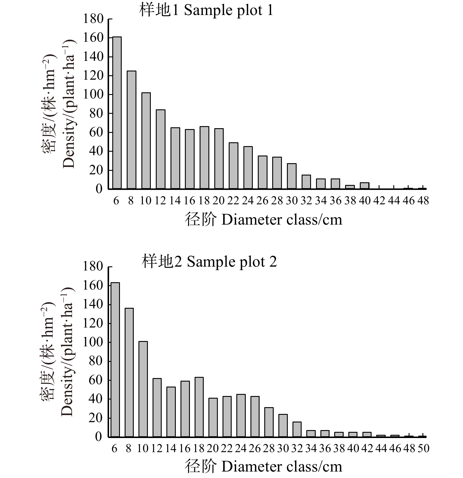
图 1 样地1和样地2活立木径级分布
Figure 1. Diameter class distribution of living trees in sample plot 1 and 2
![]()
图 2 样地1和样地2活立木高度级分布
Figure 2. Height class distribution of living treesin sample plot 1 and 2
![]()
图 3 样地1和样地2枯立木径级分布
Figure 3. Diameter class distribution of dead standing trees insample plot 1 and 2
![]()
图 4 样地1和样地2枯立木高度级分布
Figure 4. Height class distribution of dead standing trees insample plot 1 and 2
![]()
图 5 样地1和样地2活立木空间结构参数的三元分布
Figure 5. Trivariate distribution of spatial structure parameters of living trees in sample plot 1 and 2
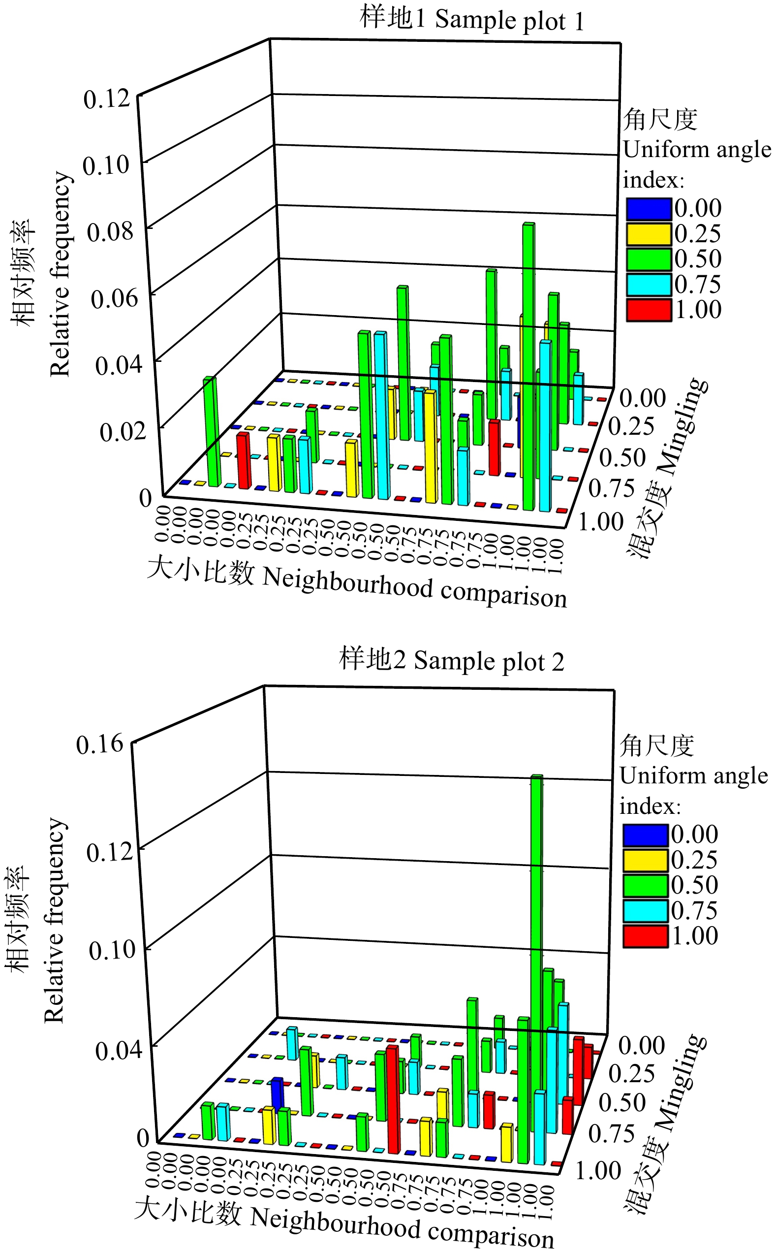
![]()
图 6 样地1和样地2枯立木空间结构参数的三元分布
Figure 6. Trivariate distribution of spatial structure parameters of dead standing trees in sample plot 1 and 2
![]()
图 7 样地1中枯立木空间结构参数的四元分布
Figure 7. Quadrivariate distribution of spatial structure parameters of dead standing trees in sample plot 1
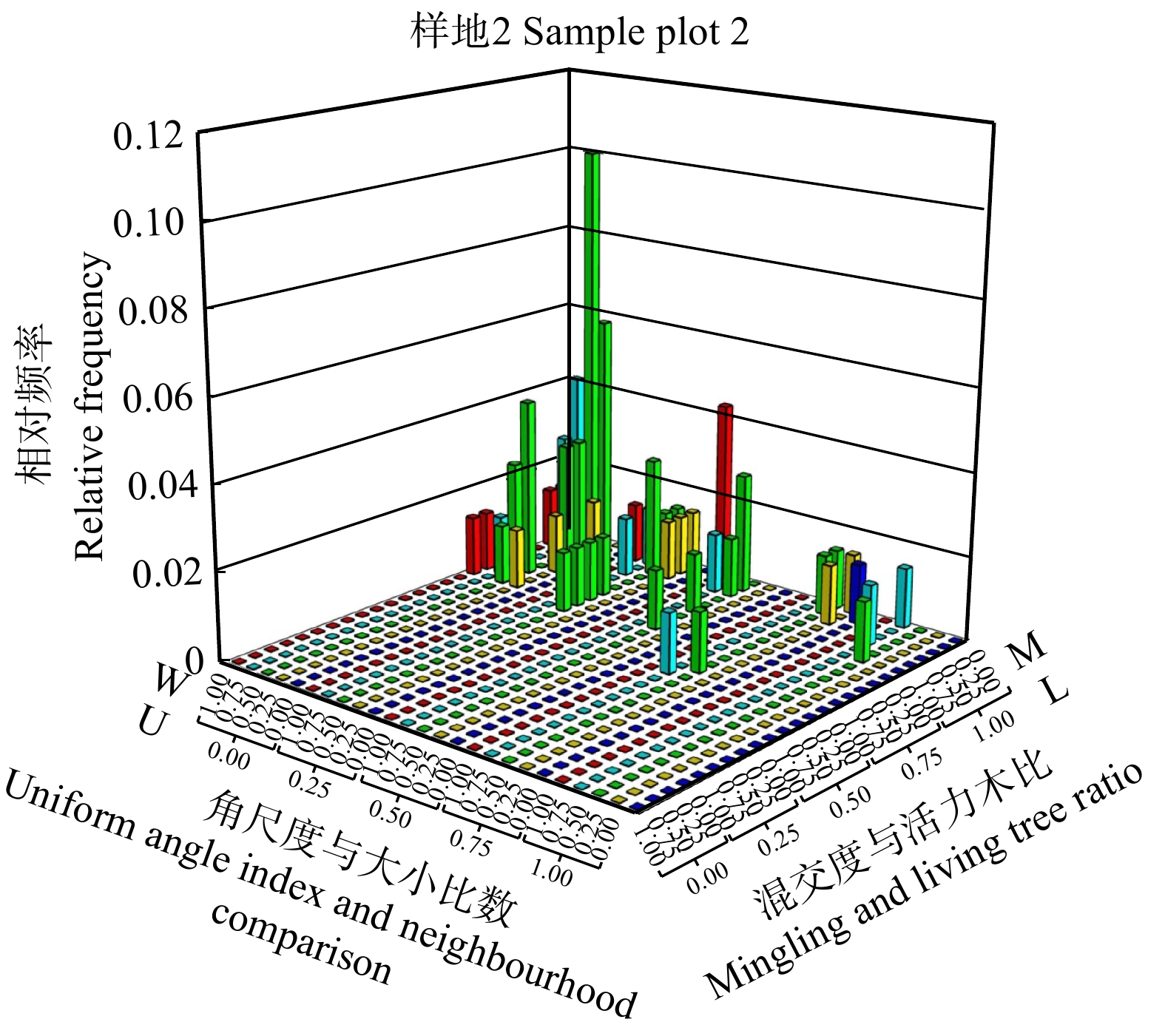
![]()
图 8 样地2中枯立木空间结构参数的四元分布
Figure 8. Quadrivariate distribution of spatial structure parameters of dead standing trees in sample plot 2
表 1 标准地基本概况
Table 1 General condition of sample plots
样地编号
Sample
plot No.坡度
Slope
degree/(°)坡向
Slope
aspect平均海拔
Average altitude/m郁闭度
Crown
density断面积/(m2·hm−2)
Basal area/
(m2·ha−1)林分平均胸径
Mean stand DBH/cm林分密度/(株·hm−2)
Stand density/
(plant·ha−1)树种组成
Tree species composition1 27 西南Southwest 378 0.80 30.4 15.1 1 291 3紫2色1蒙1白3杂 2 24 西南Southwest 420 0.84 29.8 14.7 1 235 4色3紫1糠1青1杂 注:紫为紫椴;色为色木槭;蒙为蒙古栎;白为白桦;糠为糠椴;青为青楷槭;杂为其他树种。Notes:
紫,Tilia amurensis; 色,Acer mono; 蒙,Quercus mongolica; 白,Betula platyphylla; 糠,Tilia mandshurica; 青,Acer tegmentosum; 杂,other tree species. 下载: 导出CSV
表 2 空间结构参数
Table 2 Spatial structure parameters
参数 Parameter 公式 Formula 备注 Remark 混交度 Mingling Mi=1nn∑jVij 当参照树i与第j株相邻木非同种时,Vij取值为1;否则取值为0
The value of Vij is 1 when the reference tree i is not the same species as that of the adjacent trees of strain j; otherwise, the value is 0角尺度 Uniform angle index Mi=1nn∑jZij 当第i个a角小于标准角a0时,Zij取值为1;否则取值为0
When the first angle a is smaller than the standard a0, the Zij value is 1; otherwise, the value is 0大小比数 Neighbourhood comparison Ui=1nn∑jKij 当相邻木j比参照树i小,Kij取值为0;否则取值为1
When the adjacent tree j is smaller than the reference tree i, the value of Kij is 0; otherwise, the value is 1活立木比 Living tree ratio Li=144∑j=1lij 当相邻木j为枯立木时,lij取值为0;否则取值为1
When the adjacent tree j is standing dead tree, the value of lij is 0; otherwise it’s 1
下载: 导出CSV
表 3 角尺度、混交度、大小比数和活立木比各参数的数值及意义
Table 3 Specific values and meanings of uniform angle index, mingling, dominance and living tree ratio
角尺度
Uniform angle index混交度
Mingling大小比数
Neighbourhood comparison活立木比
Living tree ratio参数值
Parameter value意义
Meaning参数值
Parameter value意义
Meaning参数值
Parameter
value意义
Meaning参数值
Parameter
value意义
MeaningW = 0.00 非常均匀
分布
Very regular distributionM = 0.00 无混交
No mixtureU = 0.00 优势状态
Predominant stateL = 0.00 参照树周围4株相邻木无活立木
4 adjacent trees around the reference tree without living treesW = 0.25 均匀分布
Regular distributionM = 0.25 低混交
Low mixtureU = 0.25 亚优势状态
Subdominant stateL = 0.25 参照树周围4株相邻木有1株活立木There is 1 living tree among 4 adjacent trees around the reference tree W = 0.50 随机分布
Random distributionM = 0.50 中度混交
Medium mixtureU = 0.50 中庸状态
Medium stateL = 0.50 参照树周围4株相邻木有2株活立木There are 2 living trees among 4 adjacent trees around the reference tree W = 0.75 团状分布
Clumped distributionM = 0.75 高度混交
High mixtureU = 0.75 中庸向劣势过渡状态
From medium to disadvantaged stateL = 0.75 参照树周围4株相邻木有3株活立木There are 3 living trees among 4 adjacent trees around the reference tree W = 1.00 聚集分布
Very clumped distributionM = 1.00 极强混交
Complete mixtureU = 1.00 劣势状态
Absolutely disadvantaged stateL = 1.00 参照树周围4株相邻木有4株活立木There are 4 living trees among 4 adjacent trees around the reference tree
下载: 导出CSV
表 4 活立木及枯立木树种组成的数量特征
Table 4 Tree species attributes of living trees and dead standing trees
样地1 Sample plot 1 样地2 Sample plot 2 树种
Tree species密度/
(株·hm− 2)
Density/
(plant·ha− 1)断面积/
(m2·hm− 2)
Basal area/
(m2·ha− 1)平均胸径
Mean DBH/
cm树种
Tree species密度/
(株·hm− 2)
Density/
(plant·ha− 1)断面积/
(m2·hm− 2)
Basal area/
(m2·ha− 1)平均胸径
Mean DBH/
cm活立木 Living
tree紫椴
Tilia amurensis529 10.089 15.781 色木槭
Acer mono485 5.777 11.865 色木槭
Acer mono323 4.246 12.463 紫椴
Tilia amurensis311 7.148 17.721 蒙古栎
Quercus mongolica70 2.331 19.212 青楷槭
Acer tegmentosum89 0.426 8.073 黄菠萝
Phellodendron amurense40 0.756 16.421 槺椴
Tilia mandshurica75 1.718 17.531 大叶榆
Ulmus laevis38 0.947 17.732 白桦
Betula platyphylla34 2.114 30.482 白桦
Betula platyphylla30 1.449 24.581 蒙古栎
Quercus mongolica28 1.373 25.313 其他
Others187 3.921 16.961 枫桦
Betula costata26 1.545 28.964 其他
Others98 2.260 18.685 枯立木
Dead standing tree紫椴
Tilia amurensis44 0.232 8.644 色木槭
Acer mono33 0.114 7.135 大叶榆
Ulmus laevis6 0.064 12.434 紫椴
Tilia amurensis29 0.193 9.123 黄菠萝
Phellodendron amurense5 0.064 13.043 青楷槭
Acer tegmentosum5 0.012 6.234 蒙古栎
Quercus mongolica5 0.018 7.491 水榆花楸
Sorbus alnifolia4 0.043 12.423 山槐
Albizia kalkora5 0.026 9.321 白桦
Betula platyphylla3 0.074 19.563 山杨
Populus davidiana5 0.016 6.974 枫桦
Betula costata3 0.078 18.134 白桦
Betula platyphylla1 0.102 35.962 胡桃楸
Juglans mandshurica3 0.006 6.426 花曲柳
Fraxinus rhynchophylla1 0.005 8.123 槺椴
Tilia mandshurica3 0.007 6.595 槺椴
Tilia mandshurica1 0.005 8.123 蒙古栎
Quercus mongolica3 0.095 21.764 青楷槭
Acer tegmentosum1 0.003 6.424 裂叶榆
Ulmus laciniate1 0.007 9.575 水曲柳
Fraxinus mandshurica1 0.006 9.264 大叶榆
Ulmus laevis1 0.086 11.312
下载: 导出CSV
-
[1] 惠刚盈, 胡艳波, 徐海, 等. 结构化森林经营[M]. 北京: 中国林业出版社, 2007. Hui G Y, Hu Y B, Xu H, et al. Structure-based forest management[M]. Beijing: China Forestry Publishing House, 2007.
[2] Zhang L J, Hui G Y, Hu Y B, et al. Spatial structural characteristics of forests dominated by Pinus tabuliformis Carr.[J/OL]. PLoS ONE, 2018, 13: e0194710 (2018−04−13)[2018−10−22]. https://doi.org/10.1371/journal.pone.0194710.
[3] Sun J, Yu X, Wang H, et al. Effects of forest structure on hydrological processes in China[J]. Journal of Hydrology, 2018, 561(1): 187−199.
[4] Oliver C D, Larson B C. Forest stand dynamics: updated edition[M]. New York: McGraw-Hill Book Company, 1996.
[5] Fang L H, Legendre P, LaFrankie J V, et al. Distribution patterns of tree species in a Malaysian tropical rain forest[J]. Journal of Vegetation Science, 1997, 8(1): 105−114. doi: 10.2307/3237248
[6] 欧光龙, 王俊峰, 肖义发, 等. 思茅松天然林单木生物量地理加权回归模型构建[J]. 林业科学研究, 2014, 27(2):213−218. Ou G L, Wang J F, Xiao Y F, et al. Modeling individual biomass of Pinus kesiya var. langbianensis natural forests by geo-graphically weighted regression[J]. Forest Research, 2014, 27(2): 213−218.
[7] 龚直文, 亢新刚, 顾丽, 等. 天然林林分结构研究方法综述[J]. 浙江林学院学报, 2009, 26(3):434−443. Gong Z W, Kang X G, Gu L, et al. Research methods on natural forest stand structure: a review[J]. Journal of Zhejiang Forestry College, 2009, 26(3): 434−443.
[8] Houghton R A. The worldwide extent of land-use change[J]. Bioscience, 1994, 44(5): 305−313. doi: 10.2307/1312380
[9] Dobson A P, Bradshaw A D, Baker A J M. Hopes for the future: restoration ecology and conservation biology[J]. Science, 1997, 277: 515−522. doi: 10.1126/science.277.5325.515
[10] 李博, 陈家宽, 沃金森. 植物竞争研究进展[J]. 植物学通报, 1998, 15(4):18−29. Li B, Chen J K, Watkinson A R. A literature review on plant competition[J]. Chinese Bulletin of Botany, 1998, 15(4): 18−29.
[11] 段仁燕, 王孝安. 太白红杉种内和种间竞争研究[J]. 植物生态学报, 2005, 29(2):242−250. doi: 10.3321/j.issn:1005-264X.2005.02.009 Duan R Y, Wang X A. Intraspecific and interspecific competition in Larix chinensis[J]. Acta Phytoecologica Sinica, 2005, 29(2): 242−250. doi: 10.3321/j.issn:1005-264X.2005.02.009
[12] Franklin J F, Shugart H H, Harmon M E, et al. Tree death as an ecological process: the causes, consequences, and variability of tree mortality[J]. Bioscience, 1987, 37(8): 550−556. doi: 10.2307/1310665
[13] Jonsson B, Kruys N, Ranius T, et al. Ecology of species living on dead wood-lessons for dead wood management[J]. Silva Fennica, 2005, 39(2): 289−309.
[14] Siitonen J. Ecology of woody debris in boreal forests forest management, coarse woody debris and saproxylic organisms: fennoscandian boreal forests as an example[J]. Ecological Bulletins, 2001 , 51(49): 11−21.
[15] Harmon M E, Franklin J F, Swanson F J, et al. Role of coarse woody debris in temperate ecosystems[J]. Advances in Ecological Research, 2004, 34(15): 159−234.
[16] Harmon M E. Carbon sequestration in forests: addressing the scale question[J]. Journal of Forestry, 2001, 99(4): 24−29.
[17] Zielonka T. When does dead wood turn into a substrate for spruce replacement?[J]. Journal of Vegetation Science, 2006, 17(6): 739−746. doi: 10.1111/j.1654-1103.2006.tb02497.x
[18] Lachat T, Brang P, Bolliger M, et al. Totholz im wald: entstehung, bedeutung und förderung[J]. Merkbl Prax, 2014, 52(1): 1−12.
[19] Junninen K, Simila M, Kouki J, et al. Assemblages of wood-inhabiting fungi along the gradients of succession and naturalness in boreal pine-dominated forests in Fennoscandia[J]. Ecography, 2006, 29(1): 75−83. doi: 10.1111/j.2005.0906-7590.04358.x
[20] Ódor P, Heilmann-Clausen J, Christensen M, et al. Diversity of dead wood inhabiting fungi and bryophytes in semi-natural beech forests in Europe[J]. Biological Conservation, 2006, 131(1): 58−71. doi: 10.1016/j.biocon.2006.02.004
[21] Uliczka H, Angelstam P. Assessing conservation values of forest stands based on specialised lichens and birds[J]. Biological Conservation, 2000, 95(3): 343−351. doi: 10.1016/S0006-3207(00)00022-7
[22] Similä M, Kouki J, Martikainen P, et al. Saproxylic beetles in managed and seminatural Scots pine forests: quality of dead wood matters[J]. Forest Ecology and Management, 2003, 174(1−3): 365−381. doi: 10.1016/S0378-1127(02)00061-0
[23] Sverdrup-Thygeson A, Gustafsson L, Kouki J, et al. Spatial and temporal scales relevant for conservation of dead-wood associ-ated species: current status and perspectives[J]. Biodiversity and Conservation, 2014, 23(3): 513−535. doi: 10.1007/s10531-014-0628-3
[24] Heilmann-Clausen J, Christensen M. Fungal diversity on decaying beech logs: implications for sustainable forestry[J]. Biodiversity and Conservation, 2003, 12(5): 953−973. doi: 10.1023/A:1022825809503
[25] Heilmann-Clausen J, Aude E, Christensen M, et al. Cryptogam communities on decaying deciduous wood: does tree species diversity matter?[J]. Biodiversity and Conservation, 2005, 14(9): 2061−2078. doi: 10.1007/s10531-004-4284-x
[26] Müller J, Bütler R. A review of habitat thresholds for dead wood: a baseline for management recommendations in European forests[J]. European Journal of Forest Research, 2010, 129(6): 981−992. doi: 10.1007/s10342-010-0400-5
[27] 国家林业局. 国家重点保护野生植物名录(第一批)[J]. 植物杂志, 1999(5):4−11. State Administration of Forestry. List of national key protected wild plant (first batch)[J]. Journal of Plants, 1999(5): 4−11.
[28] Dale M R T, Gibson D J. Spatial pattern analysis in plant ecology[J]. Quarterly Review of Biology, 2002, 15(1): 195−196.
[29] 唐杨, 陈红, 童跃伟, 等. 长白山阔叶红松林不同强度择伐后关键树种的竞争关系[J]. 应用生态学报, 2019, 30(5):1469−1478. Tang Y, Chen H, Tong Y W, et al. Competition of key tree species with selective cutting at different intensities in broadleaved-Korean pine mixed forest in the Changbai Mountain, China[J]. Chinese Journal of Applied Ecology, 2019, 30(5): 1469−1478.
[30] 许梅, 董树斌, 张德怀, 等. 北京市紫椴种群空间分布格局研究[J]. 西北农林科技大学学报(自然科学版), 2017, 45(8):81−88. Xu M, Dong S B, Zhang D H, et al. Study on spatial distribution pattern of Tilia amurensis population in Beijing[J]. Journal of Northwest A & F University, 2017, 45(8): 81−88.
[31] 张东来, 张玲. 帽儿山林区紫椴群落物种多样性、种间关系及对环境因子的响应[J]. 森林工程, 2015, 31(6):41−44, 166. doi: 10.3969/j.issn.1001-005X.2015.06.009 Zhang D L, Zhang L. atudy on species diversity, interspecific association and response to environmental factors of Tilia amurensis community in Maoer Mountain[J]. Forest Engineering, 2015, 31(6): 41−44, 166. doi: 10.3969/j.issn.1001-005X.2015.06.009
[32] 殷东生, 葛文志, 张凤海, 等. 色木槭天然次生林种群竞争关系研究[J]. 植物研究, 2012, 32(1):105−109. doi: 10.7525/j.issn.1673-5102.2012.01.005 Yin D S, Ge W Z, Zhang F H, et al. Competition relationship of populations of natural secondary Acer mono forest[J]. Bulletin of Botanical Research, 2012, 32(1): 105−109. doi: 10.7525/j.issn.1673-5102.2012.01.005
[33] 赵中华, 刘灵, 王宏翔, 等. 红花尔基沙地樟子松天然林枯立木特征分析[J]. 林业科学研究, 2017, 30(5):788−796. Zhao Z H, Liu L, Wang H X, et al.
Dead standing trees characteristics analysis of Pinus sylvestris var. mongolica natural forest in Honghuaerji[J]. Forest Research, 2017, 30(5): 788−796. [34] 张岗岗, 刘瑞红, 惠刚盈, 等. 林分空间结构参数N元分布及其诠释: 以小陇山锐齿栎天然混交林为例[J]. 北京林业大学学报, 2019, 41(4):21−31. Zhang G G, Liu R H, Hui G Y, et al. N-variate distribution and its annotation on forest spatial structural parameters: a case study of Quercus aliena var. acuteserrata natural mixed forest in Xiaolong Mountains, Gansu Province of northwestern China[J]. Journal of Beijing Forestry University, 2019, 41(4): 21−31.
[35] Pommerening A. Evaluating structural indices by reversing forest structural analysis[J]. Forest Ecology and Management, 2006, 224(3): 266−277. doi: 10.1016/j.foreco.2005.12.039
[36] 陈亚南, 杨华, 马士友, 等. 长白山2种针阔混交林空间结构多样性研究[J]. 北京林业大学学报, 2015, 37(12):48−58. Chen Y N, Yang H, Ma S Y, et al. Spatial structure diversity of semi-natural and plantation stands of Larix gmelini in Changbai Mountains, northeastern China[J]. Journal of Beijing Forestry University, 2015, 37(12): 48−58.
[37] 汤孟平, 娄明华, 陈永刚, 等. 不同混交度指数的比较分析[J]. 林业科学, 2012, 48(8):46−53. doi: 10.11707/j.1001-7488.20120808 Tang M P, Lou M H, Chen Y G, et al. Comparative analyses on different mingling indices[J]. Scientia Silvae Sinicae, 2012, 48(8): 46−53. doi: 10.11707/j.1001-7488.20120808
[38] 王宏翔. 天然林林分空间结构的二阶特征分析[D]. 北京: 中国林业科学研究院, 2017. Wang H X. Analysis of second-order characteristics of stand spatial structure of natural forests[D]. Beijing: Chinese Academy of Forestry, 2017.
[39] 万盼. 经营方式对甘肃小陇山锐齿栎天然林林分质量的影响[D]. 北京: 中国林业科学研究院, 2018. Wan P. Impacts of forest management methods on stand quality of natural Quercus aliena var. acuteserrata forest in Xiaolongshan, Gansu Province[D]. Beijing: Chinese Academy of Forestry Sciences, 2018.
[40] 白超. 空间结构参数及其在锐齿栎天然林结构动态分析中的应用[D]. 北京: 中国林业科学研究院, 2016. Bai C. Spatial structure parameters and the application on studying structure dynamics of natural Quercus aliena var. acuteserrata forest[D]. Beijing: Chinese Academy of Forestry Sciences, 2016.
[41] 卢志军, 鲍大川, 郭屹立, 等. 八大公山中亚热带山地常绿落叶阔叶混交林物种组成与结构[J]. 植物科学学报, 2013, 31(4):336−344. doi: 10.3724/SP.J.1142.2013.40336 Lu Z J, Bao D C, Guo Y L, et al. Community composition and structure of Badagongshan (BDGS) forest dynamic plot in a mid-subtropical mountain evergreen and deciduous broadleaved mixed forest, central China[J]. Plant Science Journal, 2013, 31(4): 336−344. doi: 10.3724/SP.J.1142.2013.40336
[42] Iida Y, Kohyama T S, Kubo T, et al. Tree architecture and life - history strategies across 200 co-occurring tropical tree species[J]. Functional Ecology, 2011, 25(6): 1260−1268. doi: 10.1111/j.1365-2435.2011.01884.x
[43] 马芳, 王顺忠, 冯金朝, 等. 北京东灵山暖温带落叶阔叶林枯立木与活立木空间分布格局[J]. 生态学报, 2018, 38(16):5717−5725. Ma F, Wang S Z, Feng J C, et al. Spatial distribution patterns of snag and standing trees in awarm temperate deciduous broadleaved forest in Dongling Mountain, Beijing[J]. Acta Ecologica Sinica, 2018, 38(16): 5717−5725.
[44] 陆龙龙. 长白山林区阔叶红松林不同演替阶段群落结构特征研究[D]. 吉林: 北华大学, 2019. Lu L L. Study on community structure characteristics of different succession stages of broadleaved Korean pine forest in Changbai Mountain[D]. Jilin: Beihua University, 2019.
[45] Bond-Lamberty B, Wang C, Gower S T, et al. Corrigendum: aboveground and belowground biomass and sapwood area allometric equations for six boreal tree species of northern Manitoba[J]. Canadian Journal of Forest Research, 2014, 32(8): 1441−1450.
[46] Fraver S, Jonsson B G, Jönsson M, et al. Demographics and disturbance history of a boreal old-growth Picea abies forest[J]. Journal of Vegetation Science, 2008, 19: 789−798. doi: 10.3170/2008-8-18449
[47] Eskelson B N I, Temesgen H, Hagar J C, et al. A comparison of selected parametric and imputation methods for estimating snag density and snag quality attributes[J]. Forest Ecology and Management, 2012, 272: 26−30. doi: 10.1016/j.foreco.2011.06.041
[48] Morris E C. Effect of localized placement of nutrients on root competition in selfthinning populations[J]. Annals of Botany, 1999, 78(3): 353−364.
[49] Silvertown J W. Introduction to plant population ecology[M]. New York: Longman Scientific and Technical, 1993.
[50] Ogawa K. Time-trajectory of mean phytomass and density during a course of self-thinning in a sugi (Cryptomeria japonica D. Don) plantation[J]. Forest Ecology and Management, 2005, 214(1): 104−110.
[51] Ogawa K. Relationships between mean shoot and root masses and density in an overcrowded population of hinoki (Chamaecyparis obtusa (Sieb. et Zucc.) Endl.) seedlings[J]. Forest Ecology and Management, 2005, 213(1−3): 391−398. doi: 10.1016/j.foreco.2005.04.005
[52] 周永斌, 殷有, 殷鸣放, 等. 白石砬子国家级自然保护区天然林的自然稀疏[J]. 生态学报, 2011, 31(21):6469−6480. Zhou Y B, Yin Y, Yin M F, et al. Self-thinning of natural broadleaved forests in Baishilazi Nature Reserve[J]. Acta Ecologica Sinica, 2011, 31(21): 6469−6480.
[53] Escandón A B, Susana P, Rojas R K, et al. Sprouting extends the regeneration niche in temperate rain forests: the case of the long-lived tree Eucryphia cordifolia[J]. Forest Ecology and Management, 2013, 310(1): 321−326.
[54] Travaini A, Delibes M, Ferreras P, et al. Diversity, abundance or rare species as a target for the conservation of mammalian carnivores: a case study in southern Spain[J]. Biodivers Conserv, 1997, 6(4): 529−535. doi: 10.1023/A:1018329127772
-
期刊类型引用(2)
1. 康向阳. 关于理想森林及其经营的遗传学思考. 北京林业大学学报. 2024(06): 1-9 .  本站查看
本站查看
2. 胡勐鸿,吕寻,戴小芬,李宗德,李万峰. 日本落叶松无性系种子园和优树半同胞家系苗期比较. 东北林业大学学报. 2024(12): 10-17 . 百度学术
其他类型引用(0)


计量
- 文章访问数: 1731
- HTML全文浏览量: 668
- PDF下载量: 74
- 被引次数: 2
