
Study on single tree survival model of mixed stands of Larix olgensis, Abies nephrolepis and Picea jazoensis based on mixed effect model and survival analysis method
-
摘要:目的 准确预测林木的生存和枯损是森林生长收获模型系统中十分重要的组成部分。构建基于混合效应模型和生存分析方法相结合的林木生存模型,能够提高林木枯损模型的精度。方法 以吉林省汪清林业局20块落叶松云冷杉林样地数据为例,基于生存分析方法中常用的6个时间参数分布回归模型(指数分布、Weibull分布、对数正态分布、对数Logistic分布、Gompertz分布及Gamma分布),把林分因子和立地因子作为协变量加入到模型中去,构建林木生存模型。并在此基础上考虑样地的随机效应,并与传统模型的模拟效果进行比较。结果 研究结果表明,随着单木初始胸径的增加,其枯损的风险降低,生存率提高;随着单木大于对象木断面积值的增加,其枯损的风险增加,生存率降低;随着林分密度的增加,林木枯损的概率增加,生存率降低;立地因子对林木的生存没有显著影响;6个参数分布回归模型中,Weibull分布的模拟精度最高。与固定效应模型相比,Weibull分布模型在考虑样地水平随机效应后,模型的模拟精度获得明显的提高,并且达到极显著程度。结论 在森林经营中,要提高林木的生存率,需采取科学合理的经营方法和经营时间,避免使林分的密度过大。Abstract:Objective Accurate prediction of tree mortality is a very important part of forest growth and yield model system. Constructing a tree survival model based on mixed effect model and survival analysis method can improve the precision of tree mortality model.Method Taking the data of 20 sample plots of mixed stands of Larix olgensis, Abies nephrolepis and Picea jazoensis in Wangqing Forestry Bureau of Jilin Province, northeastern China as the example, the tree mortality and survival model was constructed based on 6 parameter distribution models of survival analysis method (exponential distribution, Weibull distribution, log-normal distribution, log-Logistic distribution, Gompertz distribution, Gamma distribution), stand factor and site factor were added into the model as covariates. The sample plot’s random effect was considered and compared with the simulation effect of the traditional model.Result With the increase of initial DBH, the risk of tree mortality decreased and the survival rate increased; with the increase of BAL, the risk of mortality increased and the survival rate decreased; with the increase of stand density per hectare, the probability of tree mortality increased and the survival rate decreased; the good-fitness of Weibull distribution model was the best; compared with the fixed effect model, the simulation accuracy of Weibull distribution model was greatly improved after considering the sample plot’s random effect, and reached a very significant degree.Conclusion In forest management, if we want to improve the survival rate of trees, we should adopt scientific and reasonable management methods and management time to avoid excessive stand density.
-
光能利用效率(LUE)是指植被通过光合作用将吸收的单位光合有效辐射转换成干物质的效率[1-2]。它不仅是植物光合作用的重要生态学概念,也是利用遥感参数模型在区域尺度监测植被生产力的关键参数。光能利用率的变化能够对植被有机物的积累过程产生直接影响。光能资源与水肥等资源相比,具有无限制性、瞬时性、不可存储性等特点,因此,在一定时空范围内,植被对光能的截获吸收和利用能力的高低直接决定了生态系统的生产潜力[2]。当前,LUE广泛应用于不同尺度陆地生态系统总初级生产力(GPP)或净初级生产力(NPP)模型估算,和全球碳循环的研究中[3-6]。一些模型的比较研究表明,基于LUE的遥感模型模拟的全球净初级生产力(NPP)的平均值与其他参考模型的平均值有很大差异[7]。模型模拟结果的不确定性主要来自植被光合作用吸收的光合有效辐射和LUE[7]两个方面。此外,由于参数本身的观测和尺度变化带来的不确定性,以及模型的建立和运用范围的扩大,对结果的认识将有很大的不确定性。因此,了解LUE的生理生态基础,对于优化LUE模型和评价模型的可靠性具有重要的意义[8]。目前,对光能利用效率的研究大多集中在农田、草地和森林生态系统中[9-11],对荒漠生态系统LUE的变化特征以及影响因子的调节机理的认识非常有限[9]。因此,不同的时间尺度上环境因子对荒漠生态系统光能利用率的作用强度还需要根据实际的观测数据进一步研究探索。
已有学者研究了不同尺度(叶片、个体、种群)碳循环过程的时间动态及其调控机理,其中LUE作为量化辐射能在群落尺度上的行为参数,已受到广泛关注。研究表明在生长季保证养分充足且没有水分胁迫的条件下,LUE是一个常数[12],同时也有研究证明LUE随着植被生长发育而改变[4,9],不同植被类型的光能利用效率具有明显的时空差异[5,9]。不同时间尺度上,影响LUE的主要环境因子也有差异在不同时间尺度上其环境影响因子也变现的各不相同。在昼夜尺度上,LUE主要受到辐射、温度等[13-14]影响;季节时间尺度上,LUE主要受到LAI、温度、养分元素等[15-16]影响。
由于观测尺度的不同,光能利用效率的计算方法也各不相同。包括叶片尺度上常采用叶片光合作用仪观测法[17-18],群落尺度上常采用生物量收获发和涡度协方差方法[3],生态系统尺度上采用遥感观测法和模型反演法等[5,19]。叶片观测法一般用于控制实验,用于探究植物叶片光合作用光响应的机理过程,LUE用表观量子速率表示。生物量收获法破坏性大且耗费大量的人力物力,一般多用于农作物的研究,其缺点是不能反应短时期(小时或者日尺度)LUE的变化。遥感观测法和模型反演多用于长时间序列的大尺度研究。涡度协方差方法被许多科研工作者用来直接测量大面积生态系统物质和能量通量,而不扰动下垫面。同时,也为研究区域生态系统尺度的光合特征参数提供了途径,为估算GPP提供了一种方法,为提高区域尺度光能利用效率的准确度提供参考。涡度协方差法在时空尺度上可以与卫星遥感尺度转换相关联,使得从冠层尺度到景观水平估算LUE成为可能。
油蒿(Artemisia ordosica)广泛分布于中国西北干旱与半干旱地区,是荒漠灌木生态系统的建群种。现已有大量关于油蒿的光合作用和灌木生态系统碳水耦合的研究[20-21],但是关于油蒿灌木荒漠LUE的季节动态变化及其对环境因子响应的研究相对较少。本文运用涡度协方差方法对宁夏盐池毛乌素沙地油蒿灌木荒漠进行了全年的连续性监测,结合同步观测的气象因子,分析油蒿灌木荒漠光能利用效率在日尺度和季节尺度的变化特征及其对环境因子的响应,了解油蒿灌木荒漠光能资源利用机理,为荒漠生态系统的永续管理和沙区植被恢复提供科学参考依据。
1. 研究区概况
该研究区于宁夏盐池毛乌素沙地生态系统国家定位观测研究站(37°42′31″ N、107°13′47″ E,海拔1 560 m)。位于毛乌素沙地南缘,是黄土高原向鄂尔多斯台地、半干旱区向干旱区、干草原区向荒漠草原区、农区向牧区过渡的重要生态交错带,属于典型中温带大陆性季风气候[22-23]。多年平均空气温度8.1 ℃(1954—2004年),全年无霜期165 d。年均降雨量287 mm,其中62%集中在7—10月之间[20],年平均潜在蒸发散为2 024 mm。该区主要由活动沙丘、半固定沙丘和固定沙丘组成。主要土壤类型为灰钙土,土壤有机质含量在0.5% ~ 0.8%之间,土壤pH值在7.5 ~ 8.5之间,在土壤层1 m深度范围内的土壤总氮含量为0.15 g/kg[21]。研究区主要植被为油蒿灌木。
2. 研究方法
2.1 CO2通量和微气象因子观测
涡度相关观测系统以高度为4.2 m的观测塔为载体,主要观测仪器包括三维超声风速仪(WindMasterTM Pro,Gill Instruments Ltd,Lymington,England)和CO2/H2O闭路红外气体分析仪(IGRA;model LI-7200,LI-COR Biosciences,Lincoln,NE,USA)。
微气象数据测量仪器均设立在4.2 m的通量塔上,辐射数据由净辐射仪(CNR-4,Kipp and Zonen,Delft,the Netherlands)测量,空气温度由空气温湿度传感器(HMP45C,Campbell Scientific Ltd,USA)测量。土壤温度由安装在通量观测塔周围的土壤温度传感器(Campbell-109,Campbell Scientific Ltd,USA)测量,土壤热通量由分布在通量塔周围的5块10 cm深的土壤热通量板(HFP01,Campbell Scientific Ltd,USA)测量,土壤体积含水量分别用10、30、70和120 cm深的土壤温湿度探头(ECH2O-5TE,Decagon Devices,USA)测量,降雨量由翻斗式雨量筒(TE525MM,Campbell Scientific Inc.,USA)测量。涡度协方差系统的数据和微气象数据用CR3000(Campbell Scientific Ltd,USA)数据采集器以10 Hz频率记录,并生成30 min的平均值。
2.2 LAI与养分元素的测定
在通量塔贡献区内设置100 m × 100 m的样地,沿样地东西方向和南北方向每隔20 m设置1条样线,样地内共设置12条样线。每两条样线相交点为叶面积指数测量点,共36个点。2014年4—10月,用LAI-2000冠层分析仪每隔1周对油蒿灌木荒漠的LAI进行一次测定。样地叶面积指数计算公式为LAI = ΣLAIi/36,式中:i为第i个测量点[22]。
2014年4月,选取10个10 m × 10 m小样方,每个小样方分别选取油蒿5株,每隔一周从每株植物上取10片叶子,带回实验室,杀青并烘至恒量,将每株油蒿的取样叶子充分混合研磨,制成供试品。每隔15 d在小样方中用土钻取0 ~ 30 cm层土样,共3次重复,将每层土壤样品均匀混合并带回实验室。自然风干后,用2 mm筛过筛,制成土样进行试验。叶氮含量和土壤全氮含量均采用凯氏定氮法测定[23]。
2.3 数据处理
生态系统净碳交换(NEE)被定义为公式(1)[24]:
NEE=Fc+Fs+Vc (1) 式中:Fc是通量观测塔测得的植被上部CO2交换量,Fs是测得的冠层内部储存通量,Vc是指垂直和水平平流效应的通量。该研究区域有着均匀分布的植被下垫面,因此Vc可忽略不计。对于低矮的冠层Fs接近于0,因此Fs可忽略不计[20]。因此,
NEE=Fc (2) 本研究所用数据从2014年1月1日至2014年12月31日,期间由于仪器故障等造成36.12%数据缺失。通过剔除异常值[25]、旋转二次坐标轴[26]、消除传感器延时影响[27]、频率响应校正[28]等方法来对10 Hz数据进行了校正和质量控制。由于在夜间稳定条件下涡流不明显,导致计算出的NEE值低于夜间实际CO2通量值,因此夜间NEE(NEEnight)数据应通过摩擦风速(u*)控制和筛选,剔除掉u* < 0.18 m/s的数据[22]。经筛选后得到47.7%的有效数据,然后用5倍标准差方法剔除掉异常值。缺失数据按照时长进行插补:不足2 h的数据间隙一般采用线性插值,对于2 h ~ 7 d的数据间隔,使用邻近7 d相同时段的观测平均值,对于大于7 d的数据缺口,采用Michaelis-Menten(3)和Lloyd-Taylor方程(4)通过区分白天和晚上的NEE和Re进行插值[29-30],通过公式(5)计算出生态系统的NEP和GEP:
NEPnight=Re10Q10(Ts−10)/10 (3) NEEday=αPARAmax (4) {\rm{NEP}} = - {\rm{NEE}},\;{\rm{GEP}} = {\rm{NEP}} + {R_{\rm{e}}} (5) 式中:NEPnight为夜间生态系统净交换量,等于夜间生态系统的呼吸值Re(μmol/(m2·s)),Ts为10 cm 深的土壤温度(℃),Re10是Ts = 10 ℃时生态系统的呼吸值(μmol/(m2·s)),Q10是生态系统的呼吸敏感因子(μmol/(m2·s))。NEEday是白天生态系统净交换量(μmol/(m2·s)),α是表观量子效率(μmol/μmol),PAR是光合有效辐射,Amax是最大光合同化速率(μmol/(m2·s)),Rd是白天生态系统平均呼吸速率(μmol/(m2·s))。因为夜间测量出的NEE值就是生态系统夜间的呼吸值(自养呼吸和异养呼吸),因此通过公式(3)将Re与Q10的参数确定出来,根据白天的土壤温度计算出白天的生态系统呼吸值,考虑到植物的光合参数会受到物候和季节变化影响,因此在进行拟合和插补工作时应分别按月进行。gs运用彭曼公式计算得到:
g_{\rm{s}} = \frac{{\lambda E {\text{γ}} {g_{\rm{a}}}}}{{{\rm{\Delta }}\left( {{R_{\rm{n}}} - G} \right) - \lambda E\left( {{\rm{\Delta }} + {\text{γ}} } \right) + \rho {C_{\rm{p}}}{\rm{VPD}}{g_{\rm{a}}}}} (6) 式中:λ为汽化潜热(J/ kg);E为测量的ET值(kg/(m2· s));γ为干湿度常数(kPa/K,通常用0.066 5 kPa/℃表示);∆为饱和蒸气压差和温度之间的斜率关系(kPa/K);ga为空气动力学导度(mm/s);Cp为空气的比热容(J/(kg·K));ρ为干空气密度(kg/m3);VPD是大气饱和水汽压差(kPa);Rn是净辐射(W/m2);G是土壤热通量(W/m2)。
\frac{1}{{{g_a}}} = \frac{u}{{{u^{*2}}}} + 6.2{u^{* - 0.67}} (7) 式中:u为冠层风度;u*为测量风速。
归一化植被指数(NDVI)的计算公式[31]:
{\rm{NDVI}} = \frac{{{{{R}}_{{\rm{NIR}}}} - {R_{{\rm{VIS}}}}}}{{{R_{{\rm{NIR}}}} + {R_{{\rm{VIS}}}}}} (8) 式中:RNIR表示近红外辐射(700 ~ 3 000 nm),RVIS表示可见光辐射(380 ~ 780 nm),本文分别用太阳辐射和光合有效辐射表示RNIR和RVIS。NDVI选用了每天11:00—14:00的辐射数据计算而得[32]。
LUE的估算结果很大程度上取决于GEP和PAR间的线性或非线性(例如直角双曲线方程)关系[33-34]。目前广泛使用的光能利用效率是指太阳辐射利用400 ~ 700 nm波长(PAR,μmol/(m2·s))范围内的光合有效辐射和植物通过吸收光合有效辐射将光能转化成生物量的速率。目前LUE的估算方法很多,但是在生态系统尺度上LUE的定义为:
{\rm{LUE}} = \frac{{{\rm{GEP}}}}{{{\rm{APAR}}}} (9) 式中:GEP为总生态系统生产力(g/(m2·d)),APAR为吸收光合有效辐射(MJ/(m2·d)),本文用散射PAR(PARdif)来代替吸收光合有效辐射[35-37]。
为研究生长季内(5—10月)不同时期LUE的主要影响因子,本文分析了GEP和LUE与环境因子之间的相关性。数据统计与分析使用Matlab2014(Version 7.12.0.,The Math Works,Natick,MA,USA),作图使用OriginPro-2015完成。
3. 结果与分析
3.1 环境因子与LUE的日变化
环境因子与LUE的日变化特征如图1所示。生长季内每日平均Ta的变化范围为11.0 ~ 28.4 ℃,每日平均Ts变化范围为8 ~ 29 ℃,VPD变化范围为0.8 ~ 2.1 kPa。VPD和Ta的最低值出现在08:00,最高值出现在16:00;Ts出现明显滞后现象,最低值出现在上午10:00左右,最高值出现在下午18:00左右;gs有一个单峰,峰值稳定在14:00左右,昼夜平均变化范围为0 ~ 4.2 mm/s。PAR呈现出明显的单峰,其中峰值稳定在14:00左右。GEP呈现出单峰趋势,其中7、8月峰值在12:00左右稳定,其余月份的峰值在10:00—16:00之间稳定,中午11:00的时候达到每日最大值,总体变化趋势表现为7月 > 8月 > 6月 > 9月 > 10月 > 5月;LUE在06:00—14:00逐渐减小,14:00—19:00逐渐增大,在14:00的时候达到每日最低值(0.000 8 ~ 0.002 4 μmol/μmol),整体的变化趋势表现为9月 > 8月 > 7月 > 6月 > 5月 > 10月。
![]() 图 1 环境因子、GEP和LUE昼夜变化趋势Ta.空气温度;Ts.10 cm深土壤温度;VPD.饱和水汽压差;gs.气孔导度;PARtot.总入射光合有效辐射;PARdif.散射光合有效辐射;GEP.生态系统总生产力;LUE.光能利用效率。下同。Ta, air temperature; Ts, soil temperature of 10 cm depth; VPD, vapor pressure deficit; gs, stomatal conductance; PARtot, total incident photosynthetically active radiation; PARdif, diffuset photosynthetically active radiation; GEP, gross ecosystem productivity; LUE, light use efficiency. The same below.Figure 1. Mean diurnal variation in environmental factors and gross ecosystem production(GEP)and light use efficiency
图 1 环境因子、GEP和LUE昼夜变化趋势Ta.空气温度;Ts.10 cm深土壤温度;VPD.饱和水汽压差;gs.气孔导度;PARtot.总入射光合有效辐射;PARdif.散射光合有效辐射;GEP.生态系统总生产力;LUE.光能利用效率。下同。Ta, air temperature; Ts, soil temperature of 10 cm depth; VPD, vapor pressure deficit; gs, stomatal conductance; PARtot, total incident photosynthetically active radiation; PARdif, diffuset photosynthetically active radiation; GEP, gross ecosystem productivity; LUE, light use efficiency. The same below.Figure 1. Mean diurnal variation in environmental factors and gross ecosystem production(GEP)and light use efficiency3.2 环境因子与LUE的季节变化
图2为2014年生长季环境因子和生物因子的季节变化。油蒿灌木的日平均气温变化范围为3.4 ~ 27.6 ℃,日平均土壤温度变化范围为8.5 ~ 28.6 ℃。NDVI的变化范围为0.2 ~ 0.4。PAR从春季到夏季逐渐增加,随后降低,峰值出现在6月9日(56.6 mol/(m2·d))。年降雨总量341.9 mm,观测期降雨具有明显的季节变异,月累计降雨量9月(76.2 mm) > 7月(74.9 mm) > 8月(67.1 mm) > 6月(43.5 mm) > 10月(26.8 mm) > 5月(5.3 mm),在5月前的累计降雨量仅36.6 mm,降雨集中在7、8、9这3个月。VPD季节变化明显,在6月达到最大值,总体表现为夏季高、冬季低,变化范围为0.05 ~ 2.8 kPa。
![]() 图 2 环境和生物因子季节动态变化图NDVI. 归一化植被指数;LAI. 叶面积指数;leaf_N. 叶片N含量;soil_N. 土壤N含量;SWC10、SWC30、SWC70分别表示10、30、70 cm土壤含水量。下同。NDVI, normalized differential vegetation index; LAI, leaf area index. leaf_N, leaf N content; soil_N, soil N content. SWC10, SWC30, SWC70, represent 10, 30, 70 cm soil water content, respectively. The same below.Figure 2. Seasonal dynamics of environmental factors and biological factors
图 2 环境和生物因子季节动态变化图NDVI. 归一化植被指数;LAI. 叶面积指数;leaf_N. 叶片N含量;soil_N. 土壤N含量;SWC10、SWC30、SWC70分别表示10、30、70 cm土壤含水量。下同。NDVI, normalized differential vegetation index; LAI, leaf area index. leaf_N, leaf N content; soil_N, soil N content. SWC10, SWC30, SWC70, represent 10, 30, 70 cm soil water content, respectively. The same below.Figure 2. Seasonal dynamics of environmental factors and biological factorsGEP在7月达到最大值(图3),此时油蒿进入完全展叶期,叶面积指数达到最大,光合速率增加并达到最大,因此在7月生态系统总初级生产力达到最大值。PAR在5月达到最大值,此时油蒿处于展叶期,LAI迅速增大(图2)并随着生长季呈现递增的趋势,由于7月份以后PAR的下降速率比GEP的下降速率大,从而导致LUE在9月份达到最大值0.002 5 g/MJ,月平均LUE介于0.000 9 ~ 0.002 5 g/MJ之间,平均值为0.002 g/MJ(图3)。8月份的总生态系统生产力总值达到最大23.19 g/(m2·d)(图4),对应的LUE月总值在9月份达到最大值0.179 g/MJ,出现这种不对等增长趋势的原因主要是由于辐射的变化所导致的(图4)。
![]() 图 3 光合有效辐射、GEP和LUE季节动态变化图Figure 3. Seasonal dynamics of photosynthetically active radiation, gross ecosystem production (GEP) and light use efficiency (LUE)
图 3 光合有效辐射、GEP和LUE季节动态变化图Figure 3. Seasonal dynamics of photosynthetically active radiation, gross ecosystem production (GEP) and light use efficiency (LUE)![]() 图 4 GEP、LUE月变化Figure 4. Monthly sum dynamics of gross ecosystem production (GEP) and light use efficiency (LUE)
图 4 GEP、LUE月变化Figure 4. Monthly sum dynamics of gross ecosystem production (GEP) and light use efficiency (LUE)3.3 季节尺度上油蒿GEP和LUE对环境因子的响应
GEP与Ta、Ts和降雨量之间呈现出较好的正相关关系(图5),随着温度的增加,GEP呈现明显的递增趋势,降雨量的增加也会提高GEP的大小,SWC对GEP的变化有着72%的贡献率。随着Nsoil含量的增大,LUE表现出先减小后增大的趋势,在Nsoil达到0.24 g/kg时达到最低,Nsoil对LUE的变化有着90%的贡献率,LUE的变化还随着gs的增大呈现先减小后增大的趋势,gs对LUE的变化有着64%的贡献率,LUE的季节变化主要受到Nsoil和gs的影响。
![]() 图 5 环境因子对GEP与LUE的影响Figure 5. Relationship between light use efficiency and environmental factors at seasonal scale
图 5 环境因子对GEP与LUE的影响Figure 5. Relationship between light use efficiency and environmental factors at seasonal scale4. 讨 论
4.1 LUE的日变化以及对环境因子的响应
生长季(5—10月)LUE昼夜变化基本保持一致,呈现出先减小后增大的趋势,在14:00达到最小值,这与呼伦贝尔贝加针茅草甸草原生态系统中的光能利用效率的昼夜变化趋势基本一致[34]。LUE的昼夜变化一般受GEP和PAR昼夜变化的驱动,其中GEP的昼夜变化趋势为先增大后趋于稳定最后变小,而PAR的昼夜变化是先增大后减小的单峰趋势,并在14:00点时PAR达到最大值。光合作用是植物生长和物质积累的基础,其中光是光合作用的主导因子[38],午后高PAR常常限制植物光合作用,从而导致在昼夜尺度上LUE的变化与GEP的变化趋势正好相反。此外,夏季LUE的昼夜变化也受生态系统冠层导度(gs)的影响,夏季植物在中午时遭受高温、高辐射胁迫,此时gs达到最小,引起气孔关闭,空气阻力增加,光合作用受阻导致叶片光合速率降低[39-40],从而降低了生态系统LUE。
4.2 LUE的季节变化以及对环境因子的响应
研究区油蒿灌木荒漠光能利用效率动态随着环境变化和植被本身的生理特征的变化而变得复杂,但是LUE有着显著的季节动态特征。LUE的季节变化呈现出先增加后下降的单峰趋势,在9月份达到最大值0.002 5 g/MJ,10月份达到最低值0.000 9 g/MJ。这与内蒙古荒漠草原的光能利用效率的变化趋势一致,在8月份达到最大值0.355 g/MJ,同时最低值出现在4月份0.219 g/MJ[41]。卫亚星等[42]对青海省稀疏灌木的研究发现LUE介于0.026 ~ 0.049 g/MJ之间,最大值出现在7月份。由于7、8月份是植被的生长旺季,水热条件充足,植被覆盖率最大,此时植被的累积光物质质量也较多,吸收光合有效辐射量最大,LUE达到最大值。
植物冠层光合作用主要受冠层吸收的太阳辐射控制,植被叶片在截获入射太阳光合有效辐射进行光合作用时也具有光保护机制。植被在环境胁迫条件下(如极端高温、水分或养分亏缺、高光强等)通过降低光合作用效率[43]实现光保护过程。氮元素不仅参与植物光合作用而且是维持植物生长的重要元素,与生物圈的演替和发展紧密相关[37],Green等[15]证实了冠层总氮含量与光能利用效率之间存在显著正相关性。在低覆盖率的地表,降雨会增加土壤含水量,改变Ts,通过影响PAR[24,41]从而改变LUE的大小。VPD会通过影响植被叶片的伸展、改变叶片气孔导度从而改变光合速率来影响LUE的变化。在本研究区域内已经被证实VPD会通过影响该生态系统的碳交换过程[44],同时土壤水分的补给不足会限制半干旱草原和灌木生态系统的生产力[44-45],从而导致LUE降低。苏培玺等[46]对荒漠植物梭梭(Haloxylon ammodendron)和沙拐枣(Calligonum mongolicum)的光合作用过程研究发现,在水分条件好时光合速率明显增大,LUE明显提高。
朱文泉等[39]结合遥感数据、气象数据和实测NPP数据,系统的模拟了中国典型植被的最大光能利用效率LUEmax,得到中国灌木类型的最大光能利用效率为0.429 g/MJ。本文估算出的光能利用效率值远远低于前人的研究,可能与荒漠生态系统较小的生产力、较大的辐射值紧密相关。实际光能利用效率与环境条件的关系非常复杂,植被类型、地理位置、气候条件、植被营养状况(叶氮含量)和植被生长阶段都会影响光能利用效率的变化。
5. 结 论
本文通过研究油蒿灌木荒漠光能利用效率的昼夜和季节动态变化,明确了在不同时间尺度上LUE的主要影响因子。
(1) 在日尺度上,LUE呈现出先降低后增加的趋势,在14:00时达到最低值;LUE的日变化主要受gs和PAR的影响。
(2) 在季节尺度上,LUE呈现出先增加后降低的趋势,在9月份达到最大值,LUE的季节变化主要受土壤N含量和gs的影响。
研究还发现,LUE的大小主要取决于GEP与PAR的比值关系,在长时间尺度上通过增加土壤的养分元素,可以提高植被的光合生产能力,从而提高光能利用效率。此外,本研究主要集中在季节和生态系统尺度上,对于毛乌素沙地油蒿灌木荒漠的最大光能利用效率的定量研究还应结合卫星遥感数据与当地多年的地面实测数据相结合进行多时空多尺度的研究。
-
![]()
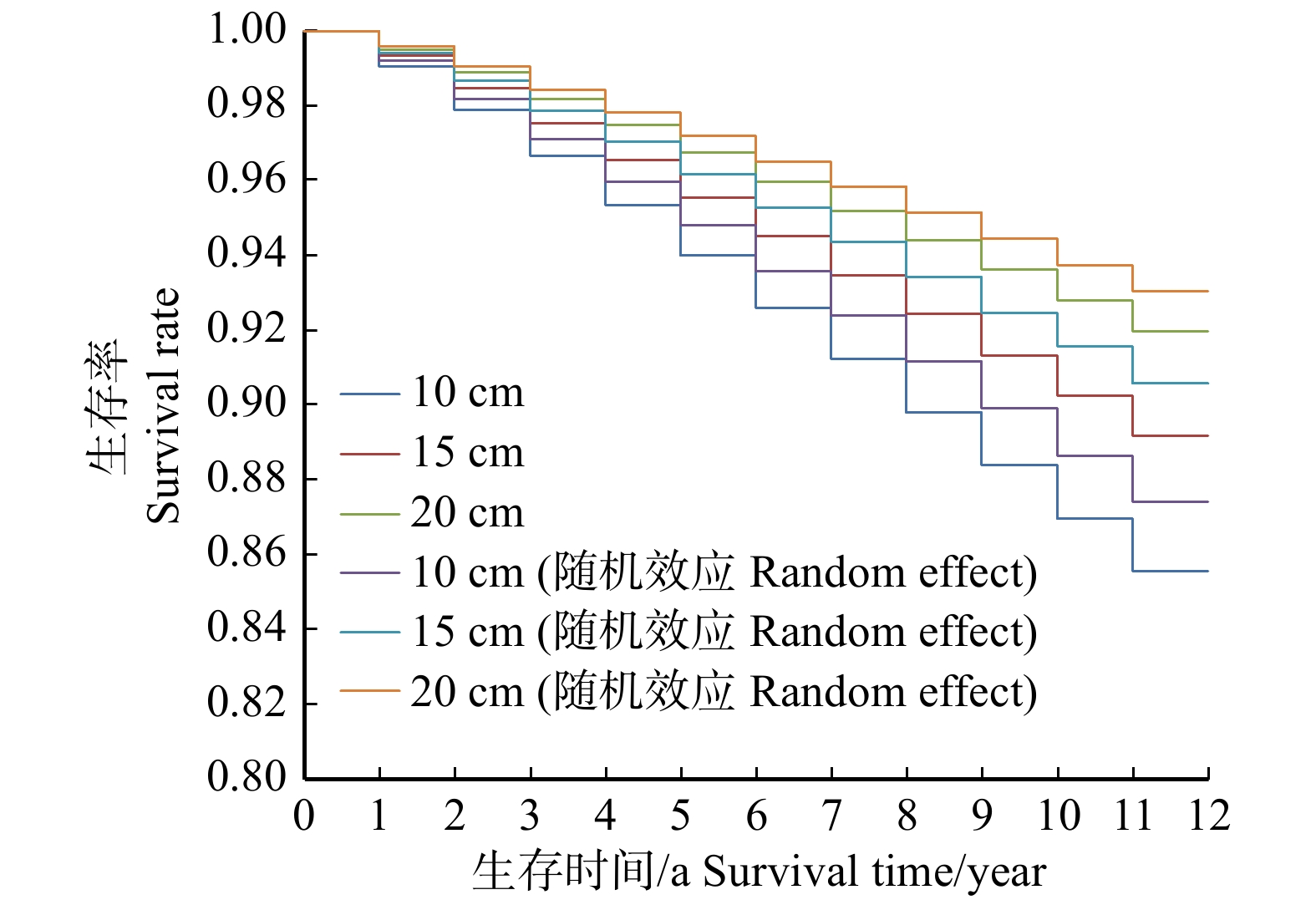
图 1 落叶松云冷杉林林木生存曲线趋势
Figure 1. Survival curve trend of mixed stands of Larix olgensis, Abies nephrolepis and Picea jazoensis
![]()
图 2 301样地不同初始胸径的林木生存曲线趋势
Figure 2. Survival curve trend of trees with different initial DBH in sample plot 301
![]()
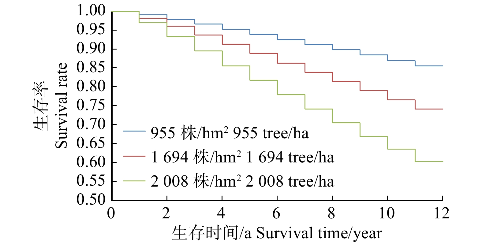
图 3 不同初值密度对胸径10 cm林木生存率的影响
Figure 3. Effect of differential initial densities on tree survival rate of 10 cm DBH
表 1 样地基本情况表
Table 1 Basic characteristics of sample plots
样地号
Sample plot No.面积/hm2
Area/ha海拔
Elevation/m坡向
Aspect坡度
Slope/(°)间伐强度
Thinning
intensity/%平均胸径
Mean DBH/
cm林分密度/
(株·hm−2)
Plant number per hectare/
(plant·ha−1)公顷断面积/
(m2·hm−2)
Basal area
per hectare/
(m2·ha−1)树种组成
Species
composition301 0.077 5 760 东北 Northeast 10 40 14.9 955 16.83 6L3PJ1PK 302 0.077 5 760 东北 Northeast 10 0 14.7 1 572 26.69 5L4PJ1K 303 0.130 0 760 东北 Northeast 10 30 14.3 1 098 17.64 4L4PJ1PK1K 304 0.097 5 760 东北 Northeast 10 20 15.9 883 17.56 7L2PJ1K 305 0.200 0 780 西 West 18 30 15.1 1 158 20.64 6L2PJ2K 306 0.200 0 780 东北 Northeast 7 0 13.7 2 008 29.42 7L2PJ1K 307 0.200 0 780 西 West 18 20 15.0 1 153 20.50 9L1K 308 0.200 0 780 东北 Northeast 10 40 15.8 846 16.39 9L1K + PJ 309 0.250 0 660 西北 Northwest 6 0 15.6 1 189 22.86 6L2PJ1PK1K 310 0.250 0 670 西北 Northwest 10 30 16.2 860 17.74 5L3PJ1PK1K 311 0.250 0 670 西北 Northwest 6 20 17.2 833 19.39 6L2PJ1K 312 0.250 0 680 西北 Northwest 10 40 15.5 914 17.30 5L2PJ2K1PK 315 0.112 5 660 北 North 7 0 13.6 1 694 24.44 6L2PJ1PK 316 0.100 0 645 北 North 7 20 14.9 1 127 19.66 6L2K1PJ1PK 317 0.100 0 615 东北 Northeast 7 20 13.5 1 286 18.65 7L2PJ1K 318 0.112 5 610 东北 Northeast 7 40 14.4 919 15.03 7L2PJ1K 319 0.100 0 605 东北 Northeast 9 30 15.2 820 14.84 10L + PK 320 0.100 0 600 东北 Northeast 9 0 13.7 1 670 24.41 6L3PJ1K 注:L. 长白落叶松; PJ. 云杉;PK. 红松;K. 包括水曲柳、白桦、椴树和枫桦等。Notes:L indicates Larix olgensis; PJ indicates Picea jazoensis; PK indicates Pinus koraiensis; K includes Fraxinus mandshurica, Betula platyphylla, Tilia tuan, Butula costata, etc.  下载: 导出CSV
表 2 各种参数分布的模型类型
Table 2 Model types of various parameter distribution
模型类型
Model type概率密度函数
Probability density function生存函数
Survival function风险函数
Hazard function指数分布 Exponential distribution (Exponential) f(t) = \lambda {{\rm{e}}^{ - \lambda t}} S(t) = {{\rm{e}}^{ - \lambda t}} h(t) = \lambda 威布尔分布 Weibull distribution (Weibull) f(t) = m\lambda {(\lambda t)^{m - 1}}{{\rm{e}}^{ - {{(\lambda t)}^m}}} S(t) = {{\rm{e}}^{ - {{(\lambda t)}^m}}} h(t) = m\lambda {(\lambda t)^{m - 1}} 对数正态分布 Log-normal distribution (log-normal) f(t) = \dfrac{1}{ {\sqrt {2\text{π} } mt} }{ {\rm{e} }^{ - 1/2{ {\left[ {(\lg t - \lambda )/m} \right]}^2} } } S(t) = 1 - \Phi \left(\dfrac{{\lg t{-}\lambda }}{m}\right) h(t) = \dfrac{ {\dfrac{1}{ {\sqrt {2\text{π} } mt} }{ {\rm{e} }^{ - 1/2{ {\left[ {(\lg t - \lambda )/m} \right]}^2} } } }}{ {1 - \Phi \left(\dfrac{ {\lg t{-}\lambda } }{m}\right)} } 对数Logistic分布 Log-Logistic distribution (log-Logistic) f(t) = \dfrac{{(m\lambda ){{(t\lambda )}^{m - 1}}}}{{{{\left[ {1 + {{(t\lambda )}^m}} \right]}^2}}} S(t) = {\left[ {1 + {{(t\lambda )}^m}} \right]^{ - 1}} h(t) = \dfrac{{(m\lambda ){{(t\lambda )}^{m - 1}}}}{{1 + {{(t\lambda )}^m}}} Gompertz分布 Gompertz distribution (Gompertz) f(t) = \lambda \exp (mt)\exp \left[ {\dfrac{\lambda }{m}(1 - {{\rm{e}}^{mt}})} \right] S(t) = \exp \left[ {\dfrac{\lambda }{m}(1 - {{\rm{e}}^{mt}})} \right] h(t) = \lambda {{\rm{e}}^{mt} } Gamma分布 Gamma distribution (Gamma) f(t) = \dfrac{{\lambda {{(\lambda t)}^{m - 1}}{{\rm{e}}^{ - \lambda t}}}}{{\Gamma (m)}} S(t) = 1 - \displaystyle\int_0^t {\dfrac{ { {t^{m - 1} }{ {\rm{e} }^{ - u} } } }{ {\Gamma (m)} }{\rm{d}}u} h[t] = \dfrac{ {\lambda { {(\lambda t)}^{m - 1} }{{\rm{e}}^{ - \lambda t} } } }{ {\Gamma (m)\left\{ {1 - F[t;T \sim \Gamma (m)]} \right\} } } 注: t 、u为时间变量, \lambda 为尺度参数, m 为形状参数。下同。Notes: t and u are time variables, \lambda is scale parameter, m is shape parameter. The same below.
下载: 导出CSV
表 3 6个参数分布模型模拟结果
Table 3 Simulation results of six parameter distribution models
参数 Parameter Exponential log-normal log-Logistic Gompertz Gamma Weibull
(固定效应Fixed effect)Weibull
(随机效应Random effect){\;\beta _0} 4.396 3
(0.159 6) ***4.168 3
(0.159 2) ***4.053 2
(0.147 0) ***4.626 7
(0.167 6) ***4.232 1
(0.149 7) ***4.218 5
(0.139 5) ***3.690 2
(0.386 5) ***{\;\beta _1} 0.051 2
(0.007 5) ***0.045 4
(0.006 9) ***0.044 8
(0.006 6) ***0.052 4
(0.007 6) ***0.046 0
(0.006 8) ***0.045 1
(0.006 6) ***0.067 7
(0.010 7) ***{\;\beta _2} −0.102 9
(0.020 9) ***−0.140 9
(0.021 0) ***−0.1239
(0.019 5) ***−0.108 9
(0.021 1) ***−0.118 7
(0.020 2) ***−0.094 3
(0.018 1) ***−0.039 6
(0.011 5) *{\;\beta _3} −0.000 6
(0.000 06) ***−0.000 6
(0.000 1) ***−0.000 6
(0.000 1) ***−0.000 7
(0.000 1) ***−0.000 6
(0.000 1) ***−0.000 6
(0.000 06) ***−0.000 4
(0.000 1) *m 1.168 8
(0.029 1)1.352 7
(0.032 7)0.018 5
(0.003 8)0.508 5
(0.103 3)1.377 3
(0.029 6)1.197 4
(0.029 7)AIC 12 973.7 12 943.4 12 947.5 12 952.3 12 952.0 12 939.1 12 697.1 BIC 12 998.3 12 974.2 12 978.3 12 983.7 12 988.9 12 969.9 12 702.9 −2logL 12 965.7 12 933.4 12 937.5 12 942.3 12 940.0 12 929.1 12 685.1 Wald {\chi ^2} < 0.001 < 0.001 < 0.001 < 0.001 < 0.001 < 0.001 < 0.001 注: {\;\beta _0} 为截距值, {\;\beta _1} 为单木初始胸径值, {\;\beta _2} 为大于对象木断面积值, {\;\beta _3} 为林分密度值;*为P < 0.05;**为P < 0.01;***为P < 0.001,括号内的数值为参数的标准差。Notes: {\;\beta _0} is intercept value, {\;\beta _1} is initial DBH of single tree, {\;\beta _2} is basal area larger than the object tree, {\;\beta _3} is value of stand density;
* means P < 0.05; ** means P < 0.01; *** means P < 0.001, values in brackets are SD of parameters.
下载: 导出CSV
-
[1] Monserud A R. Simulation of forest tree mortality[J]. Forest Science, 1976, 22: 438−444.
[2] Hamilton D A, Jr. A logistic model of mortality in thinned and unthinned mixed conifer stands of northern Idaho[J]. Forest Science, 1986, 32: 989−1000.
[3] Hann D W, Wang C H. Mortality equation for individual trees in the mixedconifer zone of southwest oregon[M]. Corvallis: Oregon State University, 1990.
[4] Adame P, del Rio M, Canellas I. Modeling individual-tree mortality in Pyrenean oak (Quercus pyrenaica Willd.) stands[J]. Annualof Forest Science, 2010, 67(8): 810−815. doi: 10.1051/forest/2010046
[5] Vanoni M, Bugmann H, Nötzli M, et al. Drought and frost contribute to abrupt growth decreases before tree mortality in nine temperate tree species[J]. Forest Ecology and Management, 2016, 382: 51−63. doi: 10.1016/j.foreco.2016.10.001
[6] Woodall C W, Grambsch P L, Thomas W. Applying survival analysis to a large-scale forest inventory for assessment of tree mortality in Minnesota[J]. Ecology Modelling, 2005, 189: 199−208. doi: 10.1016/j.ecolmodel.2005.04.011
[7] Lee Y J. Predicting mortality for even-ages stands of lodgepole pine[J]. Forestry Chronicle, 1971, 47: 29−32. doi: 10.5558/tfc47029-1
[8] Moser J W. Dynamics of an uneven-aged forest stand[J]. Forest Science, 1972, 18: 184−191.
[9] Harms W R. An empirical function for predicting survival over a wide range of densities[C]//Proceedings Second Biennial South Silvicultural Research Conference, 4–5 November 1982, Atlanta, GA. Atlanta: USDA Forest Service Gen. Tech. Rep. SE-24, 1983: 334−337.
[10] Buford M A, Hafley W L. Modeling the probability of individual tree mortality[J]. Forest Science, 1985, 31(2): 331−341.
[11] Kobe R K, Coates K D. Models of sapling mortality as a function of growth to characterize inter-specific variation in shade tolerance of eight tree species of northwestern British Columbia[J]. Canadian Journal of Forest Research, 1997, 27(2): 227−236. doi: 10.1139/x96-182
[12] Chen C, Weiskittel A, Bataineh M, et al. Even low levels of spruce budworm defoliation affect mortality and ingrowth but net growth is more driven by competition[J]. Canadian Journal of Forest Research, 2017, 47(11): 1546−1556.
[13] Zhao D, Borders B, Wang M, et al. Modeling mortality of second-rotation loblolly pine plantations in the piedmont/ upper coastal plain and lower coastal plain of the southern United States[J]. Forest Ecology and Management, 2007, 252(1−3): 132−143. doi: 10.1016/j.foreco.2007.06.030
[14] Yang Y, Huang S. A generalized mixed logistic model for predicting individual tree survival probability with unequal measurement intervals[J]. Forest Science, 2013, 59(2): 177−187. doi: 10.5849/forsci.10-092
[15] Boeck A, Dieler J, Biber P, et al. Predicting tree mortality for European beech in southern Germany using spatially explicit competition indices[J]. Forest Science, 2014, 60(4): 613−622. doi: 10.5849/forsci.12-133
[16] Eerikainen K, Miina J, Valkonen S. Models for the regeneration establishment and the development of established seedlings in uneven-aged, Norway spruce dominated forest stands of southern Finland[J]. Forest Ecology and Management, 2007, 242: 444−461. doi: 10.1016/j.foreco.2007.01.078
[17] Allison P D. Survival analysis using the SAS system, a practical guide[M]. Cary: SAS Institute, 1995.
[18] Uzoh F C C, Mori S R. Applying survival analysis to managed even-aged stands of ponderosa pine for assessment of tree mortality in the western United States[J]. Forest Ecology and Management, 2012, 285: 101−122. doi: 10.1016/j.foreco.2012.08.006
[19] Waters W E. Life-table approach to analysis of insect impact[J]. Journal of Forestry, 1969, 67: 300−304.
[20] Fan Z F, Kabrick J M, Shifley S R. Classification and regression tree based survival analysis in oak-dominated forests of Missouris Ozark highlands[J]. Canadian Journal of Forest Research, 2006, 36: 1740−1748. doi: 10.1139/x06-068
[21] von Gadow K, Kotze H, Seifert T, et al. Potential density and tree survival: an analysis based on South African spacing studies[J]. Southern Forests, 2014, 8: 1−8.
[22] 郭华, 王孝安, 王世雄, 等. 黄土高原子午岭辽东栎(Quercus liaotungensis) 幼苗动态生命表及生存分析[J]. 干旱区研究, 2011, 28(6):1005−1100. Guo H, Wang X A, Wang S X, et al. Dynamic life table and analysis on survival of Quercus liaotungensis seedlings in Mt. Ziwuling of the Loess Plateau[J]. Arid Zone Research, 2011, 28(6): 1005−1100.
[23] Manso R, Pukkala T, Pardos M, et al. Modelling Pinus pinea forest management to attain natural regeneration under present and future climatic scenarios[J]. Canadian Journal of Forest Research, 2014, 44: 250−262. doi: 10.1139/cjfr-2013-0179
[24] Franklin J F, Shugart H H, Harmon M E. Death as an ecological process: the causes, consequences, and variability of tree mortality[J]. Bioscience, 1987, 37: 550−556. doi: 10.2307/1310665
[25] Yang Y, Titus S J, Huang S. Modeling individual tree mortality for white spruce in Alberta[J]. Ecology Modelling, 2003, 163: 209−222. doi: 10.1016/S0304-3800(03)00008-5
[26] 李春明. 基于Cox比例风险函数及混合效应的落叶松云冷杉混交林林木枯损模型研究[J]. 林业科学研究, 2020, 33(3):92−98. Li C M. Mortality model of Larix olgensis-Abies nephrolepis-Picea jazoensis mixed stands based on cox proportional hazard function and mixed effect model[J]. Forest Research, 2020, 33(3): 92−98.
[27] 杜纪山. 落叶松林木枯损模型[J]. 林业科学, 1999, 35(2):45−49. doi: 10.3321/j.issn:1001-7488.1999.02.008 Du J S. Tree mortality model of Larix[J]. Scientia Silvae Sinicae, 1999, 35(2): 45−49. doi: 10.3321/j.issn:1001-7488.1999.02.008
[28] Yao X H, Titus S J, MacDonald S E. A generalized logistic model of individual tree mortality for aspen, white spruce, and lodgepole pine in Alberta mixed wood forests[J]. Canadian Journal of Forest Research, 2001, 31: 283−291.
[29] Bigler C, Bugmann H. Growth-dependent tree mortality models based on tree rings[J]. Canadian Journal of Forest Research, 2003, 33: 210−221. doi: 10.1139/x02-180
[30] Wunder J, Brzeziecki B, Zybura H, et al. Growth-mortality relationships as indicators of life-history strategies: a comparison of nine tree species in unmanaged European forests[J]. Oikos, 2008, 117: 815−828. doi: 10.1111/j.0030-1299.2008.16371.x
[31] Hurst J M, Stewart G H, Perry G L, et al. Determinants of tree mortality in mixed old-growth Nothofagus forest[J]. Forest Ecology and Management, 2012, 270: 189−199. doi: 10.1016/j.foreco.2012.01.029
[32] Timilsina N, Staudhammer C L. Individual tree mortality model for slash pine in Florida: a mixed modeling approach[J]. Southern Jounal of Apply Forest, 2012, 36(4): 211−219. doi: 10.5849/sjaf.11-026
[33] Wu H, Franklin S B, Liu J M, et al. Relative importance of density dependence and topography on tree mortality in a subtropical mountain forest[J]. Forest Ecology and Management, 2017, 384: 169−179. doi: 10.1016/j.foreco.2016.10.049
[34] Moore J A, Hamilton D A, Jr, Xiao Y, et al. Bedrock type significantly affects individual tree mortality for various conifers in the inland northwest, USA[J]. Canadian Journal of Forest Research, 2004, 34: 31−42. doi: 10.1139/x03-196
[35] Lawless J F. Statistical models and methods for lifetime data[M]. New York: John Wiley and Sons, 2003.
[36] 王建文. 生存分析参数回归模型拟合及其SAS实现[D]. 太原: 山西医科大学, 2008. Wang J W. The fitting of survival analysis and SAS implementation[D]. Taiyuan: Shanxi Medical University, 2008.
[37] Rawlings J O, Pantula S G, Dickey D A. Applied regression analysis: a research tool[M]. 2nd ed. New York: Springer, 1998.
[38] Hastie T, Tibshirani R, Friedman J. The elements of statistical learning: data mining, inference, and prediction[M]. New York: Springer, 2001.
[39] Burnham K P, Anderson D R. Model selection and multi-model inference: a practical information-theoretic approach[M]. 2nd ed. New York: Springer, 2002.
[40] 李春明. 基于两层次线性混合效应模型的杉木林单木胸径生长量模型[J]. 林业科学, 2012, 48(3):66−73. doi: 10.11707/j.1001-7488.20120311 Li C M. Individual tree diameter increment model for Chinese fir plantation based on two-level linear mixed effects models[J]. Scientia Silvae Sinicae, 2012, 48(3): 66−73. doi: 10.11707/j.1001-7488.20120311
[41] Sieg C H, Mcmillin J D, Fowler J F, et al. Best predictors for postfire mortality of ponderosa pine trees in the intermountain west[J]. Forest Science, 2006, 53(6): 718−728.
[42] Thapa R, Burkhart H E. Modeling stand-level mortality of loblolly pine (Pinus taeda L.) using stand, climate, and soil variables[J]. Forest Science, 2014, 61(5): 834−846.
[43] Ganio L M, Woolley T, Shaw D C, et al. The discriminatory ability of postfire tree mortality logistic regression models[J]. Forest Science, 2015, 61(2): 344−352. doi: 10.5849/forsci.13-146
[44] 李春明, 付卓. 基于非线性混合效应模型的3个针叶树种削度方程研究[J]. 西南林业大学学报(自然科学), 2021, 41(1):118−124. Li C M, Fu Z. The taper equation of 3 coniferous tree species based on nonlinear mixed effects models[J]. Journal of Southwest Forestry University (Natural Science), 2021, 41(1): 118−124.
[45] Hallinger M, Johansson V, Schmalholz M, et al. Factors driving tree mortality in retained forest fragments[J]. Forest Ecology and Management, 2016, 368: 163−172. doi: 10.1016/j.foreco.2016.03.023


计量
- 文章访问数: 988
- HTML全文浏览量: 404
- PDF下载量: 143
