
Comparative study on phenology in a mountainous plantation in northern China based on vegetation index, chlorophyll fluorescence and carbon flux
-
摘要:目的 物候指植被生长发育的节律性变化,是对气候和环境变化长期适应的结果。本文通过研究植被指数(NDVI、EVI)和日光诱导叶绿素荧光(SIF)与总初级生产力(GPP)之间关系,探究各指数在研究区反映植被动态变化的能力,为深入了解人工林对气候变化的响应提供参考。方法 利用Timesat 3.3软件对2007—2011年MODIS NDVI、EVI、GOME-2 SIF、通量塔GPP数据分别进行滤波。采用双逻辑斯蒂方程对4种指数时间序列进行拟合并根据曲线最大变化速率提取生长季开始期(SOS)和生长季结束期(EOS)。利用相关性分析、均方根误差分析研究NDVI、EVI、SIF反映植被动态特征的能力。结果 (1)2007—2011年MODIS NDVI、EVI、GOME-2 SIF、通量塔GPP这4种时间序列曲线变化特征基本一致,NDVI、EVI、SIF月均值均与GPP月均值呈现显著正相关关系。(2)GPP月均值与NDVI、EVI之间决定系数R2在春季、秋季均大于SIF。然而,在夏季GPP月均值与NDVI呈现显著相关性,与EVI和SIF并无明显线性关系。(3)NDVI、EVI、SIF与GPP提取物候参数的均方根误差结果显示:利用EVI提取物候参数结果与GPP最为接近,其次为NDVI,最后为SIF。结论 在本研究区内,MODIS NDVI、EVI能够更好地反映植被动态变化特征。由于NDVI、EVI数据是依据植被冠层结构光谱特性和叶片反射率提取的物候信息,因此会导致植被指数(NDVI、EVI)提取物候期比GPP提取物候开始期提前和物候结束期滞后。利用SIF数据提取物候参数SOS和EOS均提前于GPP数据提取物候参数S0S和EOS。SIF数据由于像元覆盖面积与通量塔GPP数据不完全吻合影响了GPP与SIF之间的相关关系。Abstract:Objective Phenology is the rhythmic variation of vegetation development. It is a long adapting result to climatic and environmental changes. In this study, we investigated the relationships between MODIS NDVI, EVI, GOME-2 SIF and gross primary productivity (GPP) in order to explore the ability of reflecting dynamic variation of the vegetation. This study can provide some suggestions for deep understanding the reaction of the plantation to climatic changes.Method The time series of NDVI, EVI, SIF and GPP from 2007 to 2011 were filtered using Timasat 3.3 software. Four types of index curves were fitted using double logistic functions and phenological parameters were extracted based on the maximum rate of change. Linear regression and root mean squared error (RMSE) between NDVI, EVI, SIF and GPP were used to compare the ability of reflecting the dynamic variations of the vegetation.Result (1) The time series of MODIS NDVI, EVI and GOME-2 SIF were consistent with GPP. Monthly mean NDVI, EVI and SIF were positively correlated with monthly mean GPP from 2007 to 2011. (2) The determination coefficient (R2) values between monthly mean GPP and NDVI, EVI in spring and autumn were better than that between monthly mean SIF and GPP. However, GPP was strongly correlated with NDVI in summer. The relationships between GPP and EVI, SIF were not obvious. (3) RMSE between GPP-based phenological parameters and EVI-based phenological parameters was less than that between GPP and NDVI, SIF-based phenological parameters. The order of the RMSE value was EVI, NDVI and SIF.Conclusion NDVI and EVI can better reflect the dynamic variation of the plantation in this site. The start of the growing season (SOS) extracted by MODIS NDVI and EVI advanced in comparison with the GPP-based SOS. The end of growing season (EOS) extracted by MODIS NDVI and EVI delayed in comparison with the GPP-based EOS. The main reason was that phenological information based on MODIS NDVI and EVI was extracted according to spectral characteristics of canopy structure and leaf reflectance. The SOS and EOS extracted by SIF advanced compared with the GPP-based SOS and EOS. The footprint of GOME-2 SIF mismatched with the footprint of flux tower GPP, thus impacting the relationship between SIF and GPP.
-
植被物候影响着碳和水的循环,它可以从叶和冠层结构(如:展叶)的变化或叶片和冠层功能角度(如:光合作用和总初级生产力)来确定[1]。从植被结构和功能上准确估算和比较植物物候对于改善陆地模型、探索生态系统的碳水相互作用和变化具有重要的意义[2-3]。提升估算物候变化时间信息的能力,同时把这些信息与生态系统功能变化相联系,有助于人们理解当前和未来气候与生态系统之间的相互关系[4]。
卫星遥感观测已经成为研究时间和空间上物候特征和生态系统对环境变化响应过程的一个重要手段[5]。尽管开花和结果等物候时间很难从遥感影像中识别,但它可以提供地面覆盖定期重复观测,这为全球物候研究提供了机会[6]。植被指数(归一化植被指数NDVI、增强性植被指数EVI)是最初从冠层结构角度来提取生长季开始期(SOS)和生长季结束期(EOS)的,这为植被冠层动态变化提供了信息[2, 7-9]。电磁波谱中可见光和近红外的表面反射率对植物的生长发育是很敏感的,但有些部分会受到大气和云的影响而有所衰减。因此,尽管许多卫星系统会收集每日反射率信息,但原始数据仍然需要通过数据过滤来去除噪音影响[6]。
物候是决定总初级生产力(gross primary productivity,GPP)年际变化的重要因素之一[10]。GPP可以用来估算森林生态系统生长季开始期和结束期[11-12]。研究表明,落叶林中叶片展叶、衰落时间与CO2的季节变化紧密相连[4]。Rahman等[13]研究指出通量塔观测北美北部地区各种植被类型GPP数据和MODIS EVI之间具有显著相关关系。EVI与GPP之间的关系在植被类型为落叶林时比其他植被类型存在着更紧密的对应关系[8, 13]。目前,通量塔GPP数据提取物候信息也被用来验证遥感提取的物候信息结果[11, 14-15]。Wu等[14]通过GPP数据探究NDVI提取物候信息准确性。刘啸添等[15]利用通量塔数据验证NDVI、EVI、SIF这3种指数在森林植被物候研究中的差异。
太阳诱导叶绿素荧光(SIF)是植物光合作用过程中的副产物,其可用卫星平台,如:greenhouse gasesobserving satellite(GOSAT)[16-17],global ozone monitoring experiment 2(GOME-2)[18],orbiting carbon observatory 2(OCO-2)[19]等测定。这些星载SIF数据为区域和全球尺度的光合作用估算提供了便利[16, 20]。SIF同时包含了吸收的光合有效辐射和光能利用效率的信息,为植被指数(NDVI、EVI)依据植被反射率反映植被动态变化特征提供了补充[21-22]。在森林生态系统内,GOAST和GOME-2 SIF数据与模型模拟或通量塔GPP之间有显著地正相关关系[16, 23-24]。Yang等[22]发现在落叶林通量塔GPP与日和季节遥感、地面提取SIF之间具有很高的相关性。周蕾等[25]和刘啸添等[15]利用SIF数据提取物候信息发现其能够比植被指数更好地捕捉植被动态特征。但GPP与SIF之间正相关关系会因波长、植被种类、冠层结构、时间尺度等因素影响而有所不同[26-27]。
中国人工林约占森林碳汇总量的80%[28],研究人工林物候特征有助于了解人工林生态系统对环境变化的响应过程。目前,国内有关同时结合GPP、NDVI、EVI、SIF数据对植被物候的研究比较少,且缺少有关SIF、NDVI、EVI反映植被季节变化特征能力及其与GPP之间关系的研究。本文选取黄河小浪底通量站点为主要研究区域,探究NDVI、EVI、SIF获取人工林物候特征能力,并利用通量塔总初级生产力GPP对3种指数提取物候结果进行验证和对比,以期为深入探究冠层植被物候特征研究提供参考,并为人工林的碳汇评价和管理提供理论依据。
1. 研究区概况与研究方法
1.1 研究区概况
本研究区位于河南省济源市国家林业局黄河小浪底森林生态系统定位研究站(35°01′45″N、112°28′08″E,海拔410 m)。该站位于太行山南麓,黄河流域中流地段,属暖温带亚湿润季风气候,生长季盛行东北风,全年日照时数2 367.7 h,年日照率54%,年积温5 282 °C,≥ 10 °C多年平均积温4 847 °C,年平均气温12.4 ~ 14.3 ℃,年平均降水量641.7 mm,68.3%的降水量集中于6—9月。主要植被类型为栓皮栎(Quercus variabiblis)、刺槐(Robinia pseudoacia)、侧柏(Platycladus orientalis)等。土壤主要有棕壤和石灰岩风化母质淋溶性褐土,土壤结构不良,土壤中石砾含量大,在夏季有暴雨时易受侵蚀,土层浅薄,平均40 cm,保水保肥能力差。
1.2 碳通量数据
植被物候验证数据来自于黄河小浪底森林生态系统定位研究站2007—2011年的通量观测数据。总初级生产力(GPP)是单位时间内植被通过光合作用吸收太阳能产生有机物的总量,计算公式如下:
GPP=Rec−NEE (1) 式中:GPP为总初级生产力;Rec为生态系统呼吸量;NEE净生态系统碳交换量[29];具体数据处理方法见Tong等[30]。
1.3 GOME-2叶绿素荧光数据
本研究使用搭载于MetOp-A 卫星上的GOME-2 SIF数据,数据下载地址为:http://acdb-ext.gsfc.nasa.gov/People/Joiner/my_gifs/GOME_F/GOME-F.htm。GOME-2捕获光谱范围在715 ~ 758 nm的大气顶部的地球辐射,辐射波长约为740 nm用于提取SIF数据。GOME-2 SIF数据在2013年7月之前生态足迹覆盖范围为40 km × 80 km,之后变为40 km × 40 km。本文中使用2007—2011年GOME-2 SIF(v28,3级)数据,空间分辨率为0.5° × 0.5°,时间分辨率为1个月,选择研究区域在像元中心内所对应数据,具体方法参照Joiner 等[23]。
1.4 植被指数数据
本文使用2007—2011年MODIS NDVI、EVI数据产品,下载地址为:https://ladsweb.modaps.eosdis.nasa.gov,空间分辨率为250 m,时间分辨率16 d的合成植被指数数据(MOD13Q1,collecction6,tilesH27V5)。
EVI的计算公式为:
EVI=2.5×(ρNIR−ρRρNIR+6ρR−7.5ρB+1) (2) NDVI的计算公式为:
NDVI=(ρNIR−ρR)/(ρNIR+ρR) (3) 式中:ρR、ρNIR、ρB分别代表MODIS光谱反射波段的1、2、3波段[31]。
为使研究区域与通量塔覆盖生态足迹范围相匹配,本研究中选用4 × 4像元窗口(1 km2)提取EVI、NDVI时间序列。尽管MOD13Q1数据初期已经过残留大气污染过滤处理,但数据中仍然包括由云、气溶胶和太阳高度角等所引起的噪音所导致的错误植被指数信息[32]。为排除以上因素的影响,依据MOD13Q1数据集中所提供的数据像元可靠性(data pixel reliability),剔除由于冰雪覆盖或云等影响数值(标识为2、3的数值)[15]。
1.5 物候参数提取方法
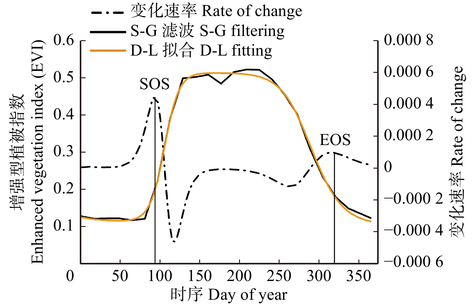
NDVI、EVI、SIF在进行拟合前使用Timesat 3.3软件对数据进行S-G滤波处理[33-34],后使用线性插值为日数据。为使结果更具有对比性,本文采用Timesat 3.3软件中所提供双逻辑斯蒂方程(double logistic functions)对GPP、NDVI、EVI、SIF时间序列分别进行数据拟合[35],公式为:
y=11+exp(t1−xt2)+11+exp(t3−xt4) (4) 式中:y为序列数据;x为数据在时间序列中所对应天数;t1、t2、t3、t4为拟合参数。
GPP、NDVI、EVI、SIF所确定的生长季开始期(the start of growing season,SOS)定义为每上半年时间序列变化速率最大值所对应的天数,生长季结束期(the end of growing season,EOS)定义为每下半年时间序列变化速率最大值所对应天数,生长季长度(the length of growing season,LOS)定义为生长季开始期到生长季结束期之间天数(图1)。
1.6 统计分析
采用线性相关法分析NDVI、EVI和SIF与GPP时间序列之间的关系。GOME-2 SIF数据时间分辨率为1个月。因此,本文均采用月数据进行线性相关分析。文中春季指3—5月、夏季指6—8月、秋季指9—11月。使用Origin2015实现数据分析和可视化。使用均方根误差(RMSE)对比NDVI、EVI、SIF提取物候参数与GPP提取物候参数之间的差异。
RMSE=√n∑i=1(ai−bi)2n (5) 式中:n为研究年份,ai为通量塔GPP提取物候参数,bi为NDVI、EVI、SIF提取物候参数。
2. 结果与分析
2.1 GPP与NDVI、EVI、SIF时间序列一致性比较
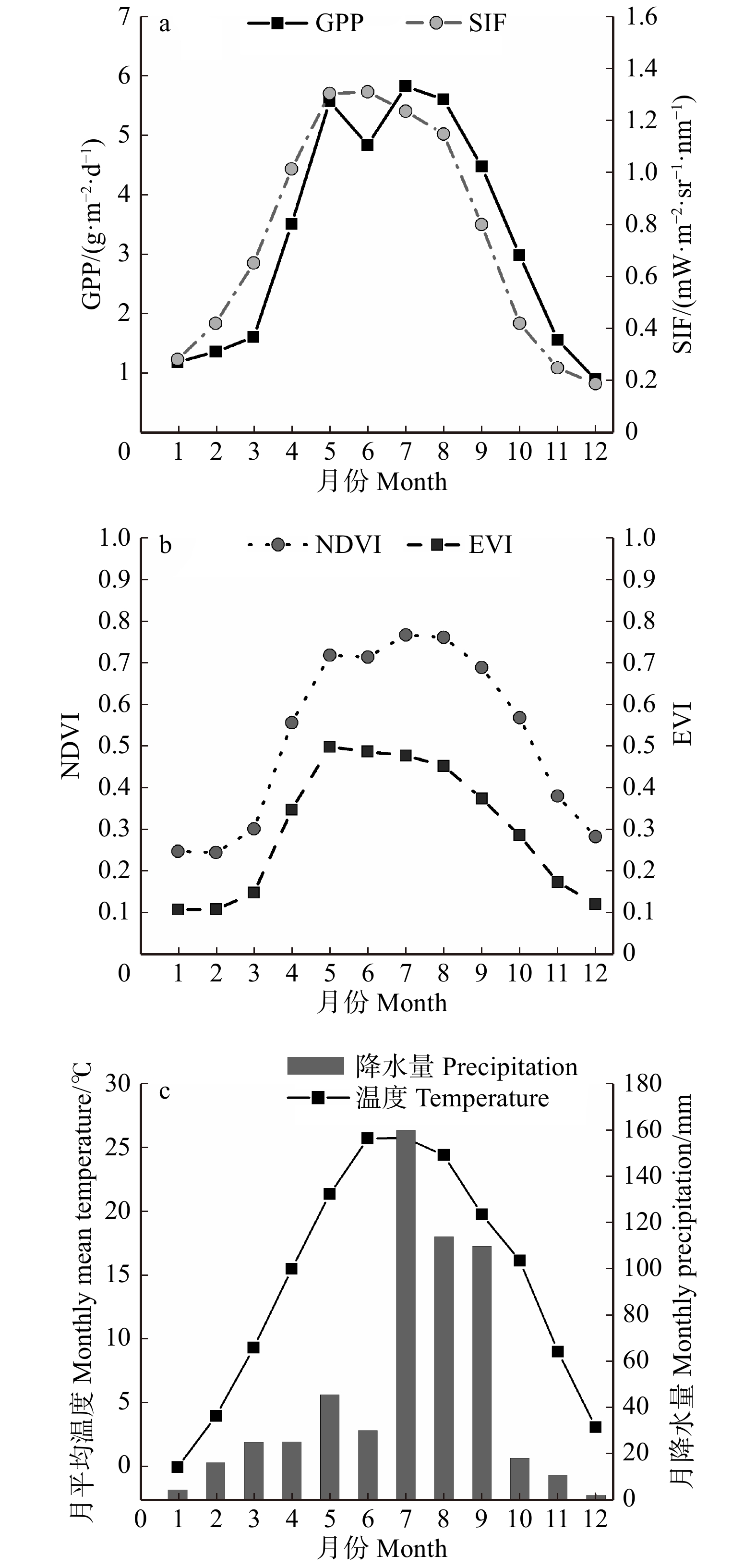
图2显示了2007—2011年4种指数时间序列变化曲线,曲线均呈现单峰状态,在生长季前后期数值均有一定程度的上下波动。受到环境因子影响,GPP、NDVI、EVI、SIF 4种时间序列曲线变化特征和温度、降水变化特征一致。随着温度升高,降水量增加,植被叶片光合作用增强,叶片绿度随之增加。从图3看出,进入春季,温度逐渐升高,曲线增长速率迅速加快。夏季温度高,降水量大,植被叶片光合作用到达顶峰,曲线数值也在夏季达到最大值。进入10月后,温度降低,降水量减少,植被叶片进入衰落期,曲线开始下降并趋于平缓。由于夏季6月份期间降水少且温度高,植被叶片光合作用减弱,导致GPP数值在6月期间有所下降。NDVI在夏季的波动特征与GPP最为接近,而EVI和SIF曲线夏季无波动特征,数值分别从5月份和6月份开始逐渐下降。在生长季前后,NDVI与EVI时间序列变化特征与GPP更为接近,而SIF时间序列生长季前期曲线上升较其他指数提前且生长季后期曲线下降较其他指数快。
![]() 图 2 2007–2011年GPP和SIF日时间序列曲线(a)、NDVI和EVI日时间序列曲线(b)和月平均温度和月降水量变化图(c)Figure 2. Seasonal variations of daily GPP and SIF time series (a), seasonal variations of daily NDVI and EVI time series (b) and monthly variations of mean temperature and precipitation (c) from 2007 to 2011
图 2 2007–2011年GPP和SIF日时间序列曲线(a)、NDVI和EVI日时间序列曲线(b)和月平均温度和月降水量变化图(c)Figure 2. Seasonal variations of daily GPP and SIF time series (a), seasonal variations of daily NDVI and EVI time series (b) and monthly variations of mean temperature and precipitation (c) from 2007 to 2011![]() 图 3 GPP和SIF(a)、NDVI和EVI(b)、以及平均温度和降水量(c)的月变化(2007—2011)Figure 3. Monthly variations of 5-year mean GPP and SIF time series (a), monthly variations of 5-year mean NDVI and EVI time series (b) and monthly variations of 5-year mean temperature and precipitation (c) (2007−2011)
图 3 GPP和SIF(a)、NDVI和EVI(b)、以及平均温度和降水量(c)的月变化(2007—2011)Figure 3. Monthly variations of 5-year mean GPP and SIF time series (a), monthly variations of 5-year mean NDVI and EVI time series (b) and monthly variations of 5-year mean temperature and precipitation (c) (2007−2011)2.2 GPP与NDVI、EVI和SIF之间的关系
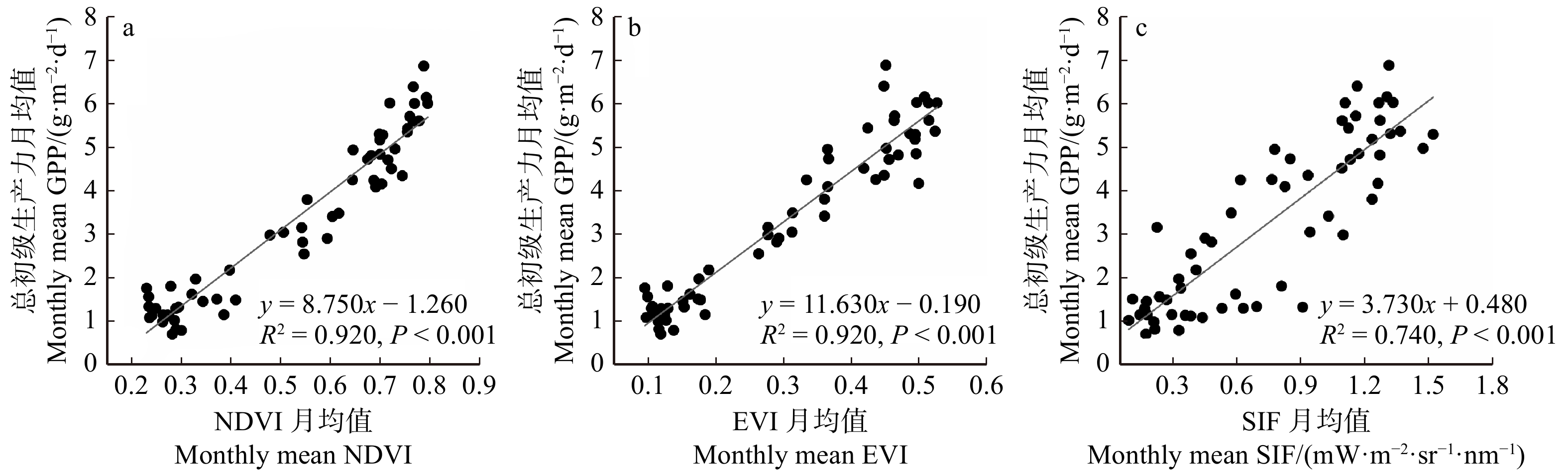
月均值相关性分析结果表明(图4),NDVI月均值、EVI月均值与GPP月均值均呈现极显著正相关关系(R2 = 0.920,P < 0.001),SIF月均值也与GPP月均值呈现极显著正相关关系(R2 = 0.740,P < 0.001),但相关性较NDVI和EVI低。在本研究区域内,NDVI和EVI能够更好地反映植被冠层动态特征。SIF因为像元覆盖面积远大于通量塔,影响了GPP与SIF的线性相关关系。图5为春季、夏季和秋季GPP月均值与其他3种指数之间的线性相关关系。春季期间,NDVI、EVI、SIF月均值与GPP月均值均呈现出显著的正相关关系(R2 = 0.950,P < 0.001;R2 = 0.960,P < 0.001;R2 = 0.560,P < 0.001)。在夏季,EVI、SIF月均值与GPP月均值并无线性相关关系(R2 = 0,P > 0.05),而NDVI与GPP之间则呈现出极显著的正相关关系(R2 = 0.720,P < 0.001)。因此,夏季NDVI能够更好地反映GPP的变化特征。秋季期间,NDVI、EVI、SIF与GPP月均值间均表现出极显著的线性相关关系。在春季和秋季,NDVI和EVI比SIF更能准确地反映植被动态变化特征。在夏季期间,NDVI能够更好的体现GPP的动态变化特征。
![]() 图 4 2007—2011年NDVI、EVI、SIF月均值与GPP月均值之间的关系Figure 4. Relationships between monthly mean GPP and NDVI, EVI, SIF from 2007 to 2011
图 4 2007—2011年NDVI、EVI、SIF月均值与GPP月均值之间的关系Figure 4. Relationships between monthly mean GPP and NDVI, EVI, SIF from 2007 to 2011![]() 图 5 2007—2011年NDVI、EVI、SIF与GPP不同季节月均值之间的关系Figure 5. Relationships between monthly mean GPP and NDVI, EVI, SIF in different seasons from 2007 to 2011
图 5 2007—2011年NDVI、EVI、SIF与GPP不同季节月均值之间的关系Figure 5. Relationships between monthly mean GPP and NDVI, EVI, SIF in different seasons from 2007 to 20112.3 物候参数结果对比分析
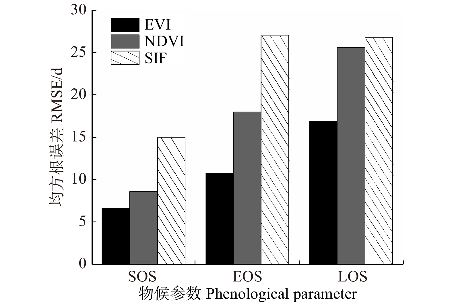
利用双逻辑斯蒂方程进行指数曲线拟合后提取物候参数结果如表1。研究区生长季开始期(SOS)主要集中在3—4月,生长季结束期(EOS)主要集中于10—11月。2007—2011年GPP、NDVI、EVI、SIF时间序列曲线提取生长季开始期(SOS)均值和标准差分别为:(91 ± 7)d、(84 ± 6)d、(86 ± 6)d、(80 ± 6)d。生长结束期(EOS)均值和标准差分别为:(309 ± 6)d、(325 ± 4)d、(316 ± 5)d、(285 ± 10)d。这表明利用NDVI、EVI、SIF提取物候生长季开始期均比GPP所得结果有所提前。对于生长季结束期,NDVI和EVI提取的物候均滞后于GPP所得结果,而SIF提取结果则明显提前于NDVI、EVI、GPP所提取的生长季结束期。4种指数提取生长季长度由大到小依次为:NDVI、EVI、GPP、SIF。对NDVI、EVI、SIF与GPP提取物候参数的均方根误差计算得出,EVI提取物候参数结果与GPP最为接近,SOS、EOS、LOS均方根误差分别为7、11、17 d,其次为NDVI(9、18、26 d),最后为SIF(15、27、27 d)(图6)。
表 1 GPP、NDVI、EVI、SIF物候参数结果对比Table 1. Comparison of phenological parameters of GPP, NDVI, EVI and SIFd 年份 Year GPP EVI NDVI SIF SOS EOS LOS SOS EOS LOS SOS EOS LOS SOS EOS LOS 2007 90 302 212 84 311 227 81 324 243 82 287 205 2008 95 301 206 82 321 239 79 326 247 68 300 232 2009 78 311 233 78 321 243 79 331 252 84 270 186 2010 97 311 214 93 310 217 92 319 227 82 279 197 2011 94 318 224 94 316 222 91 325 234 86 291 205 均值±标准差 Mean±SD 91 ± 7 309 ± 6 218 ± 10 86 ± 6 316 ± 5 230 ± 10 84 ± 6 325 ± 4 241 ± 9 80 ± 6 285 ± 10 205 ± 15 注:SOS. 生长季开始期;EOS. 生长季结束期;LOS. 生长季长度。Notes: SOS, the start of growing season; EOS, the end of growing season; LOS, the length of growing season. ![]() 图 6 NDVI、EVI、SIF提取物候参数与GPP提取物候参数之间均方根误差Figure 6. RMSE between phenological parameters extracted by GPP and those extracted by NDVI, EVI and SIF
图 6 NDVI、EVI、SIF提取物候参数与GPP提取物候参数之间均方根误差Figure 6. RMSE between phenological parameters extracted by GPP and those extracted by NDVI, EVI and SIF3. 讨 论
3.1 NDVI、EVI、SIF与GPP时间序列差异
利用遥感卫星获取SIF数据观测植被动态变化和在区域和全球尺度估算GPP是一个很有效的方法[36-37]。遥感SIF数据可以直接和独立的对不同植被类型光合作用进行估算,这是和遥感植被指数基于植被反射率是有所区别的[38-39],因此遥感所获取的SIF数据经常用来与站点通量数据GPP进行对比。Wagle 等[37]研究玉米(Zea mays )物候特征发现,GOME-2 SIF与通量塔GPP之间有极显著的相关关系,且SIF数据能够比增强型植被指数(EVI)更好地捕捉季节动态变化特征,尤其是在生长季开始期和结束期期间。Wei等[40]研究表明,GOME-2 SIF数据能够捕捉到农作物和草地地区GPP的季节动态变化特征,但是GPP与SIF之间良好线性关系依赖于SIF数据的质量以及研究区域同质性[36]。本研究发现,2007—2011年SIF月均值与GPP月均值线性相关关系(R2 = 0.740,P < 0.001)低于NDVI、EVI月均值与GPP月均值相关关系(R2 = 0.920,P < 0.001)(图4)。在春季和秋季时间尺度上,SIF月均值与GPP月均值决定系数R2范围在0.560 ~ 0.770之间,而NDVI、EVI与GPP月均值的R2范围分别是0.870 ~ 0.950和0.860 ~ 0.960,此结果也高于SIF(图5)。这是由于SIF数据的生态足迹范围(40 km × 80 km)远大于通量塔的生态足迹范围(一般为1.1 ~ 5.0 km2)[40−41]。GOME-2 SIF数据像元低分辨率,覆盖面积大导致不能与站点通量塔数据覆盖面积相吻合,且像元中可能涵盖了更多混合的地面覆盖类型[39]。同时植被冠层结构对SIF的干扰以及生物群落的组成情况也会对GPP和SIF之间的相关关系产生影响[26, 42],因为GPP的空间范围与SIF空间范围不匹配造成两者之间相关性的差异。本文同时利用MODIS NDVI、EVI、SIF数据与站点GPP数据进行相关性分析,可以更好地评估遥感数据反映植被动态特征的能力。结果表明,MODIS NDVI和EVI数据都能够良好地获取本研究区植被动态变化信息。
3.2 基于通量塔GPP、NDVI、EVI和SIF提取物候参数的比较
绿度植被指数包括NDVI和EVI已被证明是冠层参数(叶面积指数和地上植被生物量)的敏感指标[43],依次被广泛应用于提取植被物候信息[44-46]。MODIS NDVI和EVI数据可以在区域和全球尺度研究植被生长开始期、结束期和长度[47]。Wu等[14]结果表明,在落叶林研究区域内可以利用NDVI准确地估算春季和秋季物候。本文2007—2011年NDVI、EVI提取SOS,与GPP提取SOS之间的均方根误差分别为9和7 d;NDVI、EVI提取EOS,与GPP提取EOS的均方根误差分别为18和11 d(图6)。说明NDVI和EVI能够通过植被反射率角度获取春季和秋季植被动态变化特征[20, 41]。然而,利用SIF提取SOS和EOS均方根误差分别为15和27 d,低于NDVI和EVI均方根误差结果,这归因于GOME-2 SIF数据空间范围与站点通量塔所涵盖范围不匹配,限制了SIF数据反映植被动态变化的能力[36]。Li等[36]发现OCO-2 SIF数据具有更好的空间分辨率和更高的数据质量,与通量塔GPP数据之间有着更显著线性相关关系,OCO-2远红外波段SIF数据可以更好地监控植物中的光合作用。因此在以后的研究中应更多地使用不同种类的SIF数据以探究植被光合作用变化[48]。
植被指数(NDVI)数据算法中使用到红光和近红外这两种波段,而增强型植被指数EVI通过添加蓝光波段,进而改善植被覆盖率较高时红光波段所出现的饱和现象[49]。EVI对土壤背景变化不太敏感,但仍可以在茂密的植被条件下对植被冠层保持敏感性[31],因此能够更准确地获取植被动态变化信息。研究表明,与EVI相比,SIF可以更好的体现研究区域内植被动态变化特征。值得注意的是,此结果相关的大部分研究区域为冰雪覆盖区,如青海、西藏等高原地区。春季前期当冰雪消融后,以植被反射率为主的NDVI和EVI数据才能迅速升高,而SIF数据通过对植物光合作用的敏感性更好地掌握到植被的动态特征[38]。本文研究区域位于温带地区,受冰雪消融影响较小,因此EVI和NDVI可以良好地反映研究区域内的植被动态特征。
本文利用NDVI、EVI、SIF时间序列曲线提取植被物候生长期和结束期,并与GPP时间序列曲线提取物候结果进行对比,发现利用植被指数(NDVI和EVI)提取物候信息普遍提前于GPP提取生长季开始期,滞后于GPP提取生长季结束期,研究结果与牟敏杰等[29]的一致。MODIS NDVI和EVI的空间分辨率为250 m,但像元植被覆盖仍然无法完全和地面相统一。Campbell等[50]研究发现,NDVI在生长季初期会高估植被覆盖度。在生长季初期生态系统仍处于碳源阶段,植被叶片光合作用小于生态系统呼吸作用,而地面灌木及其草本植物的展叶时间提前于乔木的展叶时间,NDVI和EVI依据植被的冠层结构光谱特性和叶片反射率,可能使利用NDVI和EVI数据提取生长季开始期提前于GPP[41, 51-52]。而对于生长季结束期,乔木层植被叶片已经开始变黄和脱落,而灌木层和草本植物仍未进入衰落期[29]。叶绿素下降的过程远慢于植被光合作用逐渐降低的过程,导致了NDVI和EVI提取生长季结束期滞后于GPP提取生长季结束期[53]。
4. 结 论
本文通过对比MODIS NDVI、EVI、SIF与通量塔GPP之间关系,发现4种时间序列曲线变化特征基本一致,均可反映植被变化情况。MODIS NDVI、EVI能够更好地反映本研究区植被动态变化特征。但NDVI、EVI数据由于依据植被冠层结构光谱特性和叶片反射率提取物候信息,导致NDVI、EVI提取物候生长季开始期和结束期上存在提前和滞后现象。利用SIF数据提取SOS和EOS均提前于GPP提取物候参数。GOME-2 SIF数据由于像元时间和空间分辨率低以及覆盖面积与通量塔数据不完全吻合,限制了其反映植被动态变化的能力,影响了GPP与SIF之间的相关性。因此在以后的研究中应尽量考虑在相同空间分辨率和覆盖面积一致情况下比较不同指数之间的相关性。
-
![]()
图 2 2007–2011年GPP和SIF日时间序列曲线(a)、NDVI和EVI日时间序列曲线(b)和月平均温度和月降水量变化图(c)
Figure 2. Seasonal variations of daily GPP and SIF time series (a), seasonal variations of daily NDVI and EVI time series (b) and monthly variations of mean temperature and precipitation (c) from 2007 to 2011
![]()
图 3 GPP和SIF(a)、NDVI和EVI(b)、以及平均温度和降水量(c)的月变化(2007—2011)
Figure 3. Monthly variations of 5-year mean GPP and SIF time series (a), monthly variations of 5-year mean NDVI and EVI time series (b) and monthly variations of 5-year mean temperature and precipitation (c) (2007−2011)
![]()
图 4 2007—2011年NDVI、EVI、SIF月均值与GPP月均值之间的关系
Figure 4. Relationships between monthly mean GPP and NDVI, EVI, SIF from 2007 to 2011
![]()
图 5 2007—2011年NDVI、EVI、SIF与GPP不同季节月均值之间的关系
Figure 5. Relationships between monthly mean GPP and NDVI, EVI, SIF in different seasons from 2007 to 2011
![]()
图 6 NDVI、EVI、SIF提取物候参数与GPP提取物候参数之间均方根误差
Figure 6. RMSE between phenological parameters extracted by GPP and those extracted by NDVI, EVI and SIF
表 1 GPP、NDVI、EVI、SIF物候参数结果对比
Table 1 Comparison of phenological parameters of GPP, NDVI, EVI and SIF
d 年份 Year GPP EVI NDVI SIF SOS EOS LOS SOS EOS LOS SOS EOS LOS SOS EOS LOS 2007 90 302 212 84 311 227 81 324 243 82 287 205 2008 95 301 206 82 321 239 79 326 247 68 300 232 2009 78 311 233 78 321 243 79 331 252 84 270 186 2010 97 311 214 93 310 217 92 319 227 82 279 197 2011 94 318 224 94 316 222 91 325 234 86 291 205 均值±标准差 Mean±SD 91 ± 7 309 ± 6 218 ± 10 86 ± 6 316 ± 5 230 ± 10 84 ± 6 325 ± 4 241 ± 9 80 ± 6 285 ± 10 205 ± 15 注:SOS. 生长季开始期;EOS. 生长季结束期;LOS. 生长季长度。Notes: SOS, the start of growing season; EOS, the end of growing season; LOS, the length of growing season.  下载: 导出CSV
-
[1] Hollinger D Y, Goltz S M, Davidson E A, et al. Seasonal patterns and environmental control of carbon dioxide and water vapour exchange in an ecotonal boreal forest[J]. Global Change Biology, 1999, 5(8): 891−902. doi: 10.1046/j.1365-2486.1999.00281.x.
[2] Zhang X, Friedl M A, Schaaf C B, et al. Monitoring vegetation phenology using MODIS[J]. Remote Sensing of Environment, 2003, 84(3): 471−475. doi: 10.1016/S0034-4257(02)00135-9.
[3] 叶鑫, 周华坤, 刘国华, 等. 高寒矮生嵩草草甸主要植物物候特征对养分和水分添加的响应[J]. 植物生态学报, 2014, 38(2):147−158. doi: 10.3724/SP.J.1258.2014.00013. Ye X, Zhou H K, Liu G H, et al. Responses of phenological characteristics of major plants to nutrient and water additions in Kobresia humilis alpine meadow[J]. Chinese Journal of Plant Ecology, 2014, 38(2): 147−158. doi: 10.3724/SP.J.1258.2014.00013.
[4] Garrity S R, Bohrer G, Maurer K D, et al. A comparison of multiple phenology data sources for estimating seasonal transitions in deciduous forest carbon exchange[J]. Agricultural and Forest Meteorology, 2011, 151(12): 1741−1752. doi: 10.1016/j.agrformet.2011.07.008.
[5] Pettorelli N, Vik J O, Mysterud A, et al. Using the satellite-derived NDVI to assess ecological responses to environmental change[J]. Trends in Ecology & Evolution, 2005, 20(9): 503−510.
[6] Cleland E, Chuine I, Menzel A, et al. Shifting plant phenology in response to global change[J]. Trends in Ecology & Evolution, 2007, 22(7): 357−365.
[7] Hmimina G, Dufrêne E, Pontailler J Y, et al. Evaluation of the potential of MODIS satellite data to predict vegetation phenology in different biomes: an investigation using ground-based NDVI measurements[J]. Remote Sensing of Environment, 2013, 132: 145−158. doi: 10.1016/j.rse.2013.01.010.
[8] Sims D A, Rahman A F, Cordova V D, et al. On the use of MODIS EVI to assess gross primary productivity of North American ecosystems[J/OL]. Journal of Geophysical Research: Biogeosciences, 2006, 111: G04015 (2006−10−28) [2019−11−26]. https://10.1029/2006JG000162.
[9] Xiao X. Modeling gross primary production of temperate deciduous broadleaf forest using satellite images and climate data[J]. Remote Sensing of Environment, 2004, 91(2): 256−270. doi: 10.1016/j.rse.2004.03.010.
[10] Fu Y S H, Campioli M, Vitasse Y, et al. Variation in leaf flushing date influences autumnal senescence and next year’s flushing date in two temperate tree species[J]. Proceedings of the National Academy of Sciences, 2014, 111(20): 7355−7360. doi: 10.1073/pnas.1321727111.
[11] Baldocchi D, Falge E, Gu L, et al. FLUXNET: a new tool to study the temporal and spatial variability of ecosystem-scale carbon dioxide, water vapor, and energy flux densities[J]. Bulletin of the American Meteorological Society, 2001, 82(11): 2415−2434. doi: 10.1175/1520-0477(2001)082<2415:FANTTS>2.3.CO;2.
[12] Zhang X, Friedl M A, Schaaf C B. Global vegetation phenology from moderate resolution imaging spectroradiometer (MODIS): evaluation of global patterns and comparison with in situ measurements[J/OL]. Journal of Geophysical Research: Biogeosciences, 2006, 111: G04017 (2006−12−27) [2019−05−12]. https://10.1029/2006JG000217.
[13] Rahman A F, Sims D A, Cordova V D, et al. Potential of MODIS EVI and surface temperature for directly estimating per-pixel ecosystem C fluxes[J/OL]. Geophysical Research Letters, 2005, 32(19): L19404 (2005−10−15) [2019−12−26]. https://10.1029/2005GL024127.
[14] Wu C, Peng D, Soudani K, et al. Land surface phenology derived from normalized difference vegetation index (NDVI) at global FLUXNET sites[J]. Agricultural and Forest Meteorology, 2017, 233: 171−182. doi: 10.1016/j.agrformet.2016.11.193.
[15] 刘啸添, 周蕾, 石浩, 等. 基于多种遥感植被指数、叶绿素荧光与CO2的温带针阔混交林物候特征对比分析[J]. 生态学报, 2018, 38(10):3482−3494. Liu X T, Zhou L, Shi H, et al. Phenological characteristics of temperate coniferous and broad-leaved mixed forests based on multiple remote sensing vegetation indices, chlorophyll fluorescence and CO2 flux data[J]. Acta Ecologica Sinica, 2018, 38(10): 3482−3494.
[16] Frankenberg C, Fisher J B, Worden J, et al. New global observations of the terrestrial carbon cycle from GOSAT: patterns of plant fluorescence with gross primary productivity[J]. Geophysical Research Letters, 2011, 38(17): 351−365.
[17] Guanter L, Aben I, Tol P, et al. Potential of the TROPOspheric Monitoring Instrument (TROPOMI) onboard the sentinel-5 precursor for the monitoring of terrestrial chlorophyll fluorescence[J]. Atmospheric Measurement Techniques, 2015, 8(3): 1337−1352. doi: 10.5194/amt-8-1337-2015.
[18] Joiner J, Guanter L, Lindstrot R, et al. Global monitoring of terrestrial chlorophyll fluorescence from moderate spectral resolution near-infrared satellite measurements: methodology, simulations, and application to GOME-2[J]. Atmospheric Measurement Techniques Discussions, 2013, 6(2): 3883−3930. doi: 10.5194/amtd-6-3883-2013.
[19] Frankenberg C, O’Dell C, Berry J, et al. Prospects for chlorophyll fluorescence remote sensing from the Orbiting Carbon Observatory-2[J]. Remote Sensing of Environment, 2014, 147: 1−12. doi: 10.1016/j.rse.2014.02.007.
[20] Ma J, Xiao X, Zhang Y, et al. Spatial-temporal consistency between gross primary productivity and solar-induced chlorophyll fluorescence of vegetation in China during 2007−2014[J]. Science of The Total Environment, 2018, 639: 1241−1253. doi: 10.1016/j.scitotenv.2018.05.245.
[21] Rossini M, Nedbal L, Guanter L, et al. Red and far red sun-induced chlorophyll fluorescence as a measure of plant photosynthesis[J]. Geophysical Research Letters, 2015, 42(6): 1632−1639. doi: 10.1002/2014GL062943.
[22] Yang X, Tang J, Mustard J F, et al. Solar-induced chlorophyll fluorescence that correlates with canopy photosynthesis on diurnal and seasonal scales in a temperate deciduous forest[J]. Geophysical Research Letters, 2015, 42(8): 2977−2987. doi: 10.1002/2015GL063201.
[23] Joiner J, Yoshida Y, Vasilkov A P, et al. The seasonal cycle of satellite chlorophyll fluorescence observations and its relationship to vegetation phenology and ecosystem atmosphere carbon exchange[J]. Remote Sensing of Environment, 2014, 152: 375−391. doi: 10.1016/j.rse.2014.06.022.
[24] Walther S, Voigt M, Thum T, et al. Satellite chlorophyll fluorescence measurements reveal large-scale decoupling of photosynthesis and greenness dynamics in boreal evergreen forests[J]. Global Change Biology, 2016, 22(9): 2979−2996. doi: 10.1111/gcb.13200.
[25] 周蕾, 迟永刚, 刘啸添, 等. 日光诱导叶绿素荧光对亚热带常绿针叶林物候的追踪[J]. 生态学报, 2020, 40(12):4114−4125. Zhou L, Chi Y G, Liu X T, et al. Land surface phenology tracked by remotely sensed sun-induced chlorophyll fluorescence in subtropical evergreen coniferous forests[J]. Acta Ecologica Sinica, 2020, 40(12): 4114−4125.
[26] Damm A, Guanter L, Verhoef W, et al. Impact of varying irradiance on vegetation indices and chlorophyll fluorescence derived from spectroscopy data[J]. Remote Sensing of Environment, 2015, 156: 202−215. doi: 10.1016/j.rse.2014.09.031.
[27] Guanter L, Frankenberg C, Dudhia A, et al. Retrieval and global assessment of terrestrial chlorophyll fluorescence from GOSAT space measurements[J]. Remote Sensing of Environment, 2012, 121: 236−251. doi: 10.1016/j.rse.2012.02.006.
[28] Fang J. Changes in forest biomass carbon storage in China between 1949 and 1998[J]. Science, 2001, 292: 2320−2322. doi: 10.1126/science.1058629.
[29] 牟敏杰, 朱文泉, 王伶俐, 等. 基于通量塔净生态系统碳交换数据的植被物候遥感识别方法评价[J]. 应用生态学报, 2012, 23(2):319−327. Mou M J, Zhu W Q, Wang L L, et al. Evaluation of remote sensing extraction methods for vegetation phenology based on flux tower net ecosystem carbon exchange data[J]. Chinese Journal of Applied Ecology, 2012, 23(2): 319−327.
[30] Tong X, Meng P, Zhang J, et al. Ecosystem carbon exchange over a warm-temperate mixed plantation in the lithoid hilly area of the North China[J]. Atmospheric Environment, 2012, 49: 257−267. doi: 10.1016/j.atmosenv.2011.11.049.
[31] Huete A, Didan K, Miura T, et al. Overview of the radiometric and biophysical performance of the MODIS vegetation indices[J]. Remote Sensing of Environment, 2002, 83(1): 195−213.
[32] Ma X, Huete A, Yu Q, et al. Spatial patterns and temporal dynamics in savanna vegetation phenology across the North Australian Tropical Transect[J]. Remote Sensing of Environment, 2013, 139: 97−115. doi: 10.1016/j.rse.2013.07.030.
[33] Jönsson P, Eklundh L. Seasonality extraction by function fitting to time-series of satellite sensor data[J]. IEEE Transactions on Geoscience and Remote Sensing, 2002, 40(8): 1824−1832. doi: 10.1109/TGRS.2002.802519.
[34] Jönsson P, Eklundh L. TIMESAT: a program for analyzing time-series of satellite sensor data[J]. Computers & Geosciences, 2004, 30(8): 833−845.
[35] Jönsson P, Eklundh L. TIMESAT 3.3 with seasonal trend decomposition and parallel processing software manual[R]. Sweden: Lund and Malmö University, 2017.
[36] Li X, Xiao J, He B. Chlorophyll fluorescence observed by OCO-2 is strongly related to gross primary productivity estimated from flux towers in temperate forests[J]. Remote Sensing of Environment, 2018, 204: 659−671. doi: 10.1016/j.rse.2017.09.034.
[37] Wagle P, Zhang Y, Jin C, et al. Comparison of solar-induced chlorophyll fluorescence, light-use efficiency, and process-based GPP models in maize[J]. Ecological Applications, 2016, 26(4): 1211−1222.
[38] Qiu B, Li W, Wang X, et al. Satellite-observed solar-induced chlorophyll fluorescence reveals higher sensitivity of alpine ecosystems to snow cover on the Tibetan Plateau[J]. Agricultural and Forest Meteorology, 2019, 271: 126−134. doi: 10.1016/j.agrformet.2019.02.045.
[39] Zhang Y, Xiao X, Jin C, et al. Consistency between sun-induced chlorophyll fluorescence and gross primary production of vegetation in North America[J]. Remote Sensing of Environment, 2016, 183: 154−169. doi: 10.1016/j.rse.2016.05.015.
[40] Wei X, Wang X, Wei W, et al. Use of sun-induced chlorophyll fluorescence obtained by OCO-2 and GOME-2 for GPP estimates of the Heihe River Basin, China [J/OL]. Remote Sensing, 2018, 10(12): 2039 (2018−12−01) [2019−03−22]. https://10.3390/rs101220039.
[41] Peng D, Wu C, Li C, et al. Spring green-up phenology products derived from MODIS NDVI and EVI: intercomparison, interpretation and validation using National Phenology Network and AmeriFlux observations[J]. Ecological Indicators, 2017, 77: 323−336. doi: 10.1016/j.ecolind.2017.02.024.
[42] Zhang Y, Guanter L, Berry J A, et al. Estimation of vegetation photosynthetic capacity from space-based measurements of chlorophyll fluorescence for terrestrial biosphere models[J]. Global Change Biology, 2014, 20(12): 3727−3742. doi: 10.1111/gcb.12664.
[43] Garonna I, De Jong R, De Wit A J W, et al. Strong contribution of autumn phenology to changes in satellite-derived growing season length estimates across Europe (1982−2011)[J]. Global Change Biology, 2014, 20(11): 3457−3470. doi: 10.1111/gcb.12625
[44] 宋富强, 邢开雄, 刘阳, 等. 基于MODIS/NDVI的陕北地区植被动态监测与评价[J]. 生态学报, 2011, 31(2):354−363. Song F Q, Xing K X, Liu Y, et al. Monitoring and assessment of vegetation variation in northern Shanxi based on MODIS/NDVI[J]. Acta Ecologica Sinica, 2011, 31(2): 354−363.
[45] 夏浩铭, 李爱农, 赵伟, 等. 2001—2010年秦岭森林物候时空变化遥感监测[J]. 地理科学进展, 2015, 34(10):1297−1305. doi: 10.18306/dlkxjz.2015.10.010. Xia H M, Li A N, Zhao W, et al. Spatiotemporal variations of forest phenology in the Qinling Zone based on remote sensing monitoring[J]. Progress in Geography, 2015, 34(10): 1297−1305. doi: 10.18306/dlkxjz.2015.10.010.
[46] 于信芳, 庄大方. 基于MODIS NDVI数据的东北森林物候期监测[J]. 资源科学, 2006, 28(4):111−117. doi: 10.3321/j.issn:1007-7588.2006.04.023. Yu X F, Zhuang D F. Monitoring forest phenophases of Northeast China based on MODIS NDVI Data[J]. Resources Science, 2006, 28(4): 111−117. doi: 10.3321/j.issn:1007-7588.2006.04.023.
[47] Jeong S, Ho C, Gim H, et al. Phenology shifts at start vs. end of growing season in temperate vegetation over the northern Hemisphere for the period 1982−2008[J]. Global Change Biology, 2011, 17(7): 2385−2399. doi: 10.1111/j.1365-2486.2011.02397.x.
[48] Frankenberg C, Drewry D, Geier S, et al. Remote sensing of solar induced chlorophyll fluorescence from satellites, airplanes and ground-based stations[J/OL]. Geoscience & Remote Sensing Symposium, 2016 (2016−07−10) [2019−12−26]. https://ieeexplore.ieee.org/document/7729436.
[49] 范德芹, 赵学胜, 朱文泉, 等. 植物物候遥感监测精度影响因素研究综述[J]. 地理科学进展, 2016, 35(3):304−319. doi: 10.18306/dlkxjz.2016.03.005. Fan D Q, Zhao X S, Zhu W Q, et al. Review of influencing factors of accuracy of plant phenology monitoring based on remote sensing data[J]. Progress in Geography, 2016, 35(3): 304−319. doi: 10.18306/dlkxjz.2016.03.005.
[50] Campbell J B. Introduction to remote sensing[M]. 4th ed. New York: Guilford Press, 2007.
[51] Badeck F, Bondeau A, Böttcher K, et al. Responses of spring phenology to climate change[J]. New Phytologist, 2004, 162: 295−309. doi: 10.1111/j.1469-8137.2004.01059.x.
[52] Donnelly A, Yu R, Liu L, et al. Comparing in-situ leaf observations in early spring with flux tower CO2 exchange, MODIS EVI and modeled LAI in a northern mixed forest[J/OL]. Agricultural and Forest Meteorology, 2019, 278: 107673 (2019−07−28) [2020−02−16]. https://www.sciencedirect.com/science/article/pii/S0168192319302874.
[53] Huemmrich K F, Privette J L, Mukelabai M, et al. Time-series validation of MODIS land biophysical products in a Kalahari woodland, Africa[J]. International Journal of Remote Sensing, 2005, 26(19): 4381−4398. doi: 10.1080/01431160500113393.
-
期刊类型引用(3)
1. 裴薇薇,杨喆,王云英,王新,杜岩功. 祁连山区青海云杉林碳汇特征及调控因子. 中国农业科技导报. 2024(01): 226-233 .  百度学术
百度学术
2. 苏远航,张峰源,刘滨辉. 小兴安岭森林植被物候对气候变化的响应. 北京林业大学学报. 2023(03): 34-47 . 本站查看
3. 解晗,同小娟,李俊,张静茹,刘沛荣,于裴洋. 2000—2018年黄河流域生长季植被指数变化及其对气候因子的响应. 生态学报. 2022(11): 4536-4549 . 百度学术
其他类型引用(3)


计量
- 文章访问数: 1998
- HTML全文浏览量: 968
- PDF下载量: 177
- 被引次数: 6
