
Analysis on flower color of common garden plants in Beijing parks based on bees visual system
-
摘要:目的 蜂类是城市传粉昆虫的主要类群,具有重要的生态服务功能,而人类活动和城市发展导致蜂类数量与多样性下降。本研究基于蜂类视觉模型,评估分析各花色特征与蜂类招引能力的关系,为建立蜂类友好型园林植物的筛选体系和保护城市蜂类传粉昆虫奠定基础。方法 以奥林匹克森林公园、海淀公园、朝阳公园等6个北京市内公园的常用园林植物为研究对象,从蜂类视觉的角度,通过光谱仪测量花反射光谱,并结合蜂类视觉模型,分析了春季与夏秋季开花的园林植物的花色多样性、花色与背景的对比度等色彩特征。结果 不同季节和不同色系开花植物的色彩特征存在显著性差异。春季开花植物的花色标记点平均绝对偏差和最小绝对偏差(400 nm)显著低于夏秋季,表明春季开花植物比夏秋季开花植物更易被蜂类识别,但春季花色多样性较低。比较了白色系、黄色系、红色系、粉色系和蓝紫色系植物花色特征,发现黄色系花色多样性最高,红色系花色多样性最低。比较了不同色系的平均绝对偏差和最小绝对偏差,发现黄色系、白色系和粉色系开花植物易被蜂类识别,红色系开花植物难被蜂类识别。结论 花色光谱标记点偏差、非彩色对比度和彩色对比度能够作为筛选蜂类友好型园林植物的指标。Abstract:Objective Bees, the main species of urban pollinators, have significant ecological service function. However, human activities and urbanization had led to a decline in the number and diversity of pollinators. Based on the bees vision model, we assessed the influence of floral color characteristics on the bees-attracted ability. The results could be useful for establishing a selecting indicator system for bees-friendly landscape plants and lay a foundation for maintaining the stability of urban ecosystem.Method Taking the commonly used landscape plants in six green spaces of Beijing as the research objects, we used the floral reflectance spectrum measured by a spectrometer and bees vision model to analyze the floral characteristics, including color diversity and contrast against the background of flowering plants in spring and summer-autumn.Result There were significant differences in the floral characteristics of flowering plants of different seasons and color systems. The mean absolute deviation and minimum absolute deviation (400 nm) of spring blooming plants were significantly lower than those of summer-autumn blooming plants, indicating that the spring blooming plants were easier to be perceived, while the floral color diversity of the spring blooming plants was lower. Moreover, comparing the flower color characteristics of white, yellow, red, pink, and blue-purple flower plants, we observed that the floral color diversity was high for yellow flower plants and low for the red ones. The values of mean absolute deviation and minimum absolute deviation indicated that yellow, white and pink flower plants were easy to be perceived, whereas it was hard for bees to perceive red flower plants.Conclusion The deviation value of floral color spectral marker-points, achromatic contrast against background and chromatic contrast against background could be used as indicators for selecting bees-friendly landscape plants.
-
Keywords:
- bees /
- pollinator /
- floral color /
- bees vision /
- landscape plant
-
城市中的传粉昆虫具有重要且不可替代的传粉功能及生态补偿价值[1]。膜翅目(Hymenoptera)、鞘翅目(Coleoptera)、双翅目(Diptera)等是传粉昆虫主要类群[2],其中,膜翅目的蜂类是城市重要传粉昆虫之一。城市发展和人类活动导致的栖息地破坏是传粉昆虫数量下降的主要原因[3]。研究表明,野生蜂类在北京昌平区的自然林生境和东部的人工林中均有较高的相对多样性,而在高度城市化的非生境区域几乎不出现[4]。影响蜂类种群年数量变化的一个重要原因是蜜粉源条件,而城市公园应用的园林植物可提供蜜粉源,因此具有一定的蜂类招引能力[5-6],通过在城市公园种植蜂类友好型园林植物可为其提供生境条件,维持蜂类种群发展。
植物开花信号招引传粉昆虫访花,主要包括视觉信号(花色和花形)和嗅觉信号(花香)[7]。不同开花信号可对传粉昆虫形成单独刺激,也可通过更为复杂的相互作用形成组合刺激[8]。植物花香通常在招引昆虫长距离传粉中发挥重要作用[9],也会增强花朵招引力从而影响传粉昆虫的访花偏好[10]。植物花色是传粉综合特征中最显著的花部特征[11],也是与传粉昆虫感知和偏好有关的特征中最容易被识别的一类信号[12]。花色作为视觉信号既可单独招引传粉者,也可结合特定嗅觉信号或者花分泌物(比如花蜜和花粉)共同招引传粉昆虫。值得注意的是,传粉昆虫的颜色感知能力与人类有较大差异,其在紫外波段具有更强的感知能力[13],因此需要建立对应的视觉模型进行研究。近年来,膜翅目、双翅目、鳞翅目(Lepidoptera)主要传粉昆虫的视觉模型已被广泛运用于传粉昆虫花色感知的研究中[14]。根据对蜂类视觉系统的研究,可以将其感知的花色视觉信号分为非彩色信号、彩色信号和其他暂不明确功能的信号[15]。非彩色信号主要包括花色亮度对比度和绿色对比度,即花色与背景的亮度差异和花色与背景植被的绿色反射率差异。彩色信号主要包括色彩对比度,即蜂类所有感光细胞所感受的视觉信号总和的对比度,与色相和饱和度的差异有关。与其他传粉昆虫类似,蜂类显示出对特定色相的偏好[16-20],说明花色是招引蜂类的关键信号之一。
长期以来,蜂类友好型园林植物的选择常基于生产经验,缺少科学依据,导致目前园林中应用的此类植物存在种类单一、功能性弱的问题。因此,本研究从蜂类视觉的角度出发,明确北京公园常用园林植物花色多样性的组成特点,量化探讨各项花色特征指标与蜂类招引能力的相关性,为后续蜂类友好型植物的筛选提供参考,并为营建多功能园林植物群落和保护城市蜂类奠定基础。
1. 研究区域、材料与方法
1.1 研究区域
选择园林植物种类较丰富的北京市内6个公园作为研究区域,包括奥林匹克森林公园、海淀公园、朝阳公园、八家郊野公园、玉东郊野公园和北京植物园。
1.2 研究材料
本研究共收集到100个不同花色、花期植物样本。其中,春季开花植物(花期3—5月)39种,样本数N = 42;夏秋季开花植物(花期5—10月)40种,样本数N = 56;春季和夏秋均开花植物2种,样本数N = 2。根据研究材料的花色特点,参考Shrestha等[21]的研究,并结合计算机辅助判断将植物花色分为白色系、粉色系、红色系、黄色系、蓝紫色系。同种不同色系的开花植物记为不同样本,同种同色系不同花色的开花植物也记为不同样本,对于不同花期的植物分别进行采样与分析。
1.3 测定项目与方法
1.3.1 花反射光谱
在每处调查样地中(样地大小为1 m × 1 m),分别选择间隔0.5 m以上的3株植物[22],取植物花瓣后,放入装有冰袋的保温盒中暂时保存,尽快带回实验室进行测量。将花瓣平铺固定于黑卡纸上,确保其舒展无褶皱。参考相关研究[23-25],测量花瓣在300 ~ 700 nm波长区间内的反射光谱。该区间包括紫外区域、光谱蓝色、光谱绿色和光谱红色,涵盖了包括蜂类在内的常见传粉者的视觉范围。使用的仪器设备有Avantes AvaSpec-ULS1024LTEC微型光谱仪、安装固定在反射探头支架(RPH-1)上的标准型光纤反射探头(FCR-7UV200-2-ME-SR),Avantes AvaLight-D(H)-S氘卤钨灯组合光源。另外,使用硫酸钡标准白板来校准光谱仪。当花瓣有多种颜色时,对整花面积最大的颜色进行测量。当单花太小难以获得读数时,将多个花无间隙地平铺后进行测量[26]。
1.3.2 蜂类视觉模型
目前研究蜂类视觉主要用颜色六边形模型(color hexagon model,CH)[27],包括昆虫光感受器光谱敏感度函数、标准日光照明辐照度基准函数、背景物光谱反射率及研究对象的光谱反射率[28]。蜂类具有紫外光感受器、绿色光感受器、蓝色光感受器,分别对350、440和540 nm波段的光有高敏感度。在波长接近400 nm与500 nm的区域时,蜂类具有较强的颜色辨别能力[29]。CH模型的计算参考Ohashi的方法[14],以标准绿叶为背景,将蜂类感知的颜色差异转换为欧几里得距离。所得的距离以六边形单位(hexagon units,Hu)表示,代表两种颜色在蜂类视觉中的差异度。
1.3.3 花反射光谱特征分析
花色多样性:为了定量比较不同季节或不同花色系开花植物的花色多样性,参考Tai等[30]的计算方法,用R包SP计算同一季节或同一花色系中所有开花植物的颜色位点的最小凸多边形(minimum convex polygon,MCP)面积,该值可以在一定程度上衡量样本的花色多样性。使用最远距离法衡量整体数据离散程度,逐一剔除距离所有位点中心最远的5%的点,观察不同利用概率下的MCP面积。
标记点及特征值:在花光谱反射率曲线上发生快速变化的波长称为拐点或标记点,用于评估传粉者与花色间的互作关系[31-33],标记点的位置可以用于确定花的潜在招引对象。标记点与最佳颜色识别能力对应波长之间的平均绝对偏差(mean absolute deviation,MAD)和标记点与最佳颜色识别能力对应波长的最小绝对偏差(minimum absolute deviation,minAD)可量化花色与蜂类视觉识别能力的关系[34-36]。选择minAD400与minAD500作为蜂类识别的统计标准。为了标准化数据,使用Spectral-MP软件计算标记点[37]。
花色与背景的对比度:参考相关研究[38-44],根据光谱反射曲线计算蜜蜂视觉中有关显著性的两个参数:相对于背景的非彩色对比度(achromatic contrast against the background,ACB)和相对于背景的彩色对比度(chromatic contrast against the background,CCB)。ACB是指蜂类绿色光感受器所感知到的目标与背景间的特异性兴奋值,CCB是指目标与背景之间的颜色差异。在多种花色信号中,与背景之间的对比度是蜂类区分和检测花朵的最重要指标之一[45-46]。
1.4 数据分析
标记点及特征值和花色与背景的对比度不满足正态分布,采用单因素方差分析的K-W检验,Duncan法进行多重比较,来分析不同花色开花植物的显著性差异。
2. 结果与分析
2.1 开花植物的花色标定
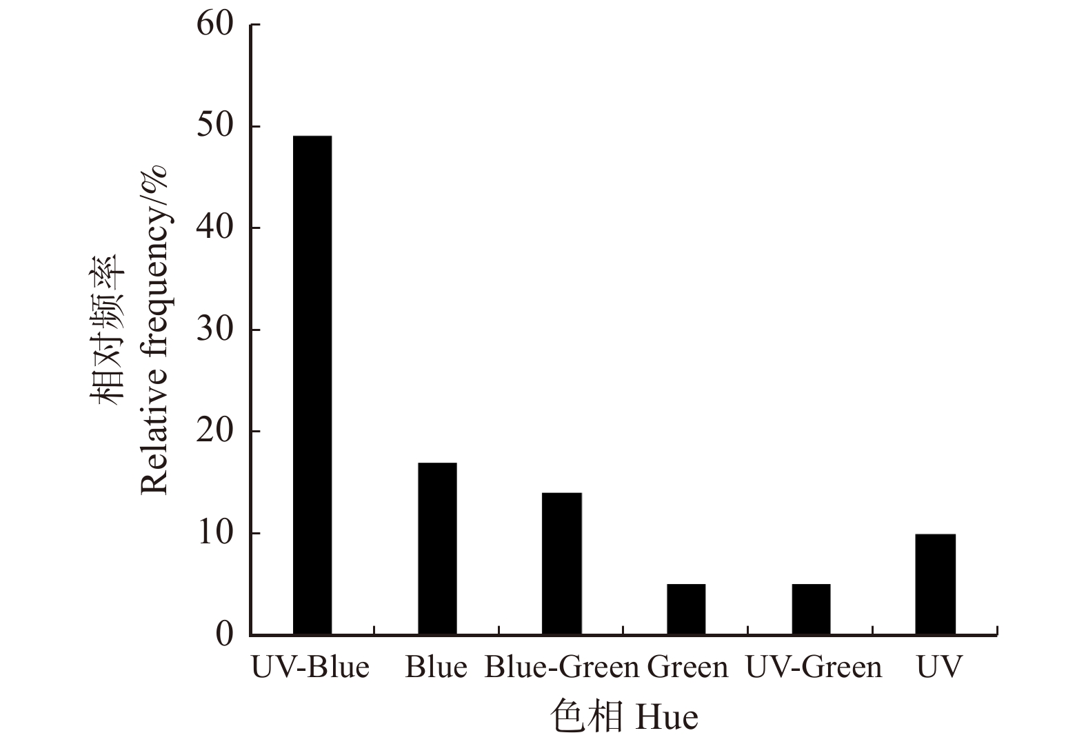
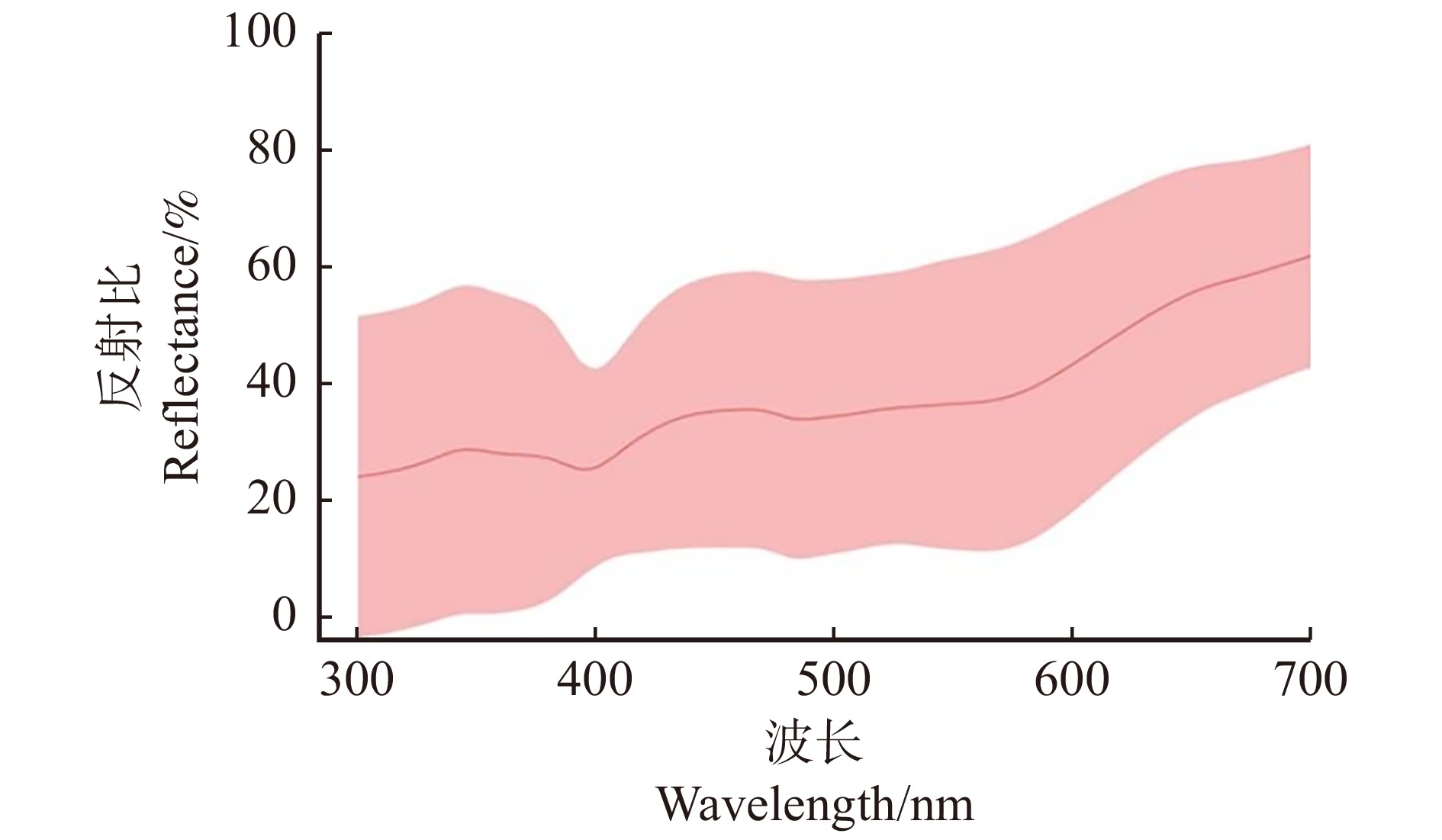
所有开花植物的花色在300 ~ 700 nm的反射比如图1所示。花颜色标定后在蜂类视觉颜色空间中的色彩位点如图2所示,各位点距中心的距离代表了对应花色与绿叶背景在蜂类视觉中的差异程度。根据各色彩点位在CH模型中的位置,将其归为对应的色相并做统计。由图3可得,在调查到的北京常见园林植物中,属于UV-Blue色相的开花植物最多(49.00%),其次是Blue(17.00%)、Blue-Green(14.00%)、UV(10.00%)色相的开花植物,属于Green和UV-Green的植物最少(5.00%)。
![]() 图 1 开花植物在波长300 ~ 700 nm的反射比红色曲线为取中位数后的反射曲线,浅红色范围为标准偏差。The red curve is the reflection curve after taking the median, and the light red range represents the standard deviation.Figure 1. Total reflectance at wavelength 300−700 nm of the flowering plants
图 1 开花植物在波长300 ~ 700 nm的反射比红色曲线为取中位数后的反射曲线,浅红色范围为标准偏差。The red curve is the reflection curve after taking the median, and the light red range represents the standard deviation.Figure 1. Total reflectance at wavelength 300−700 nm of the flowering plants![]() 图 2 开花植物在蜂类视觉颜色空间中的色彩位点六边形的6个扇区分别表示不同的蜂类视觉颜色。EB、EG、EUV分别代表蓝色光、绿色光和紫外光感受器的相对刺激值。The six sectors of the hexagon represent different color types of bees version. EB, EG, EUV represent the relative stimulus values of blue light, green light, and UV receptors, respectively.Figure 2. Color loci in bees space of the flowering plants
图 2 开花植物在蜂类视觉颜色空间中的色彩位点六边形的6个扇区分别表示不同的蜂类视觉颜色。EB、EG、EUV分别代表蓝色光、绿色光和紫外光感受器的相对刺激值。The six sectors of the hexagon represent different color types of bees version. EB, EG, EUV represent the relative stimulus values of blue light, green light, and UV receptors, respectively.Figure 2. Color loci in bees space of the flowering plants2.2 不同季节开花植物的花色分析
2.2.1 花色的标定与多样性分析
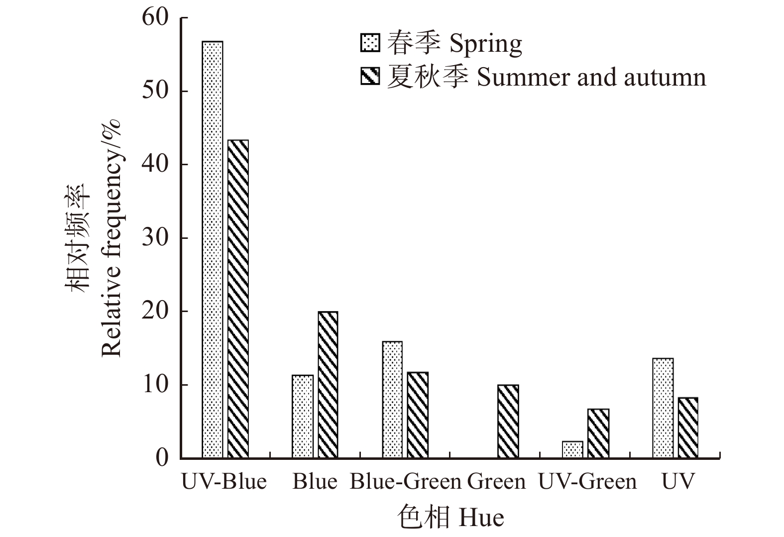
根据春季与夏秋季开花植物的色彩点位在CH模型中的位置,将其归为对应的色相并做统计。春季开花植物中,属于UV-Blue色相的植物有56.81%,属于Blue-Green、UV、Blue色相的植物分别有15.90%、13.64%和11.36%,仅有2.27%的植物属于UV-Green色相,没有植物属于Green色相。夏秋季开花植物中,属于UV-Blue色相的植物为43.33%,属于Blue、Blue-Green、Green、UV和UV-Green的植物分别为20.00%、11.67%、10.00%、8.33%和6.67%。两个采样季中,均是属于UV-Blue色相的植物最多(图4)。
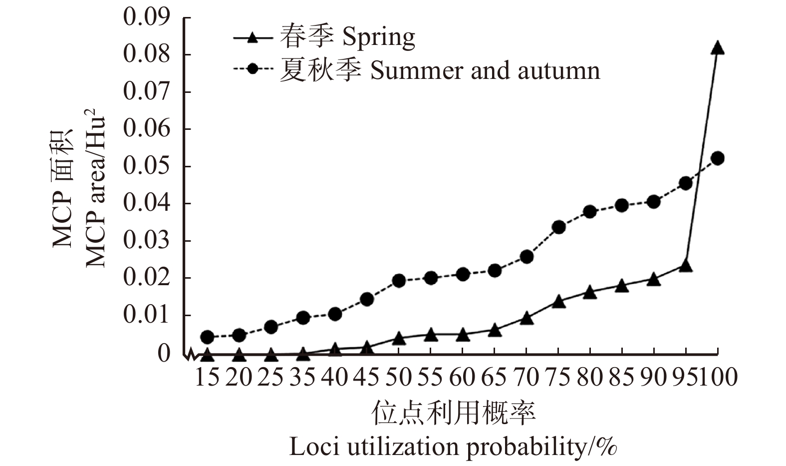
比较花色多样性,计算不同取样季的MCP面积(图5)。除了个别花色位点,春季开花植物的MCP值均小于夏秋季,说明春季开花植物的花色多样性较小,即在蜂类视觉中差异较小,夏秋季开花植物花色多样性较大,即在蜂类视觉中颜色差异较大。
![]() 图 5 不同季节植物色彩位点MCP面积MCP. 最小凸多边形。不同点位利用概率表示落在MCP内的色彩位点百分比,依次排除距离所有点位中心最远的点。MCP, minimum convex polygon. The point utilization probability represents the percentage of color loci in the MCP, and the points farthest from the centers of all points are excluded in turn.Figure 5. MCP area of plant color loci in different seasons
图 5 不同季节植物色彩位点MCP面积MCP. 最小凸多边形。不同点位利用概率表示落在MCP内的色彩位点百分比,依次排除距离所有点位中心最远的点。MCP, minimum convex polygon. The point utilization probability represents the percentage of color loci in the MCP, and the points farthest from the centers of all points are excluded in turn.Figure 5. MCP area of plant color loci in different seasons2.2.2 标记点分布特征分析
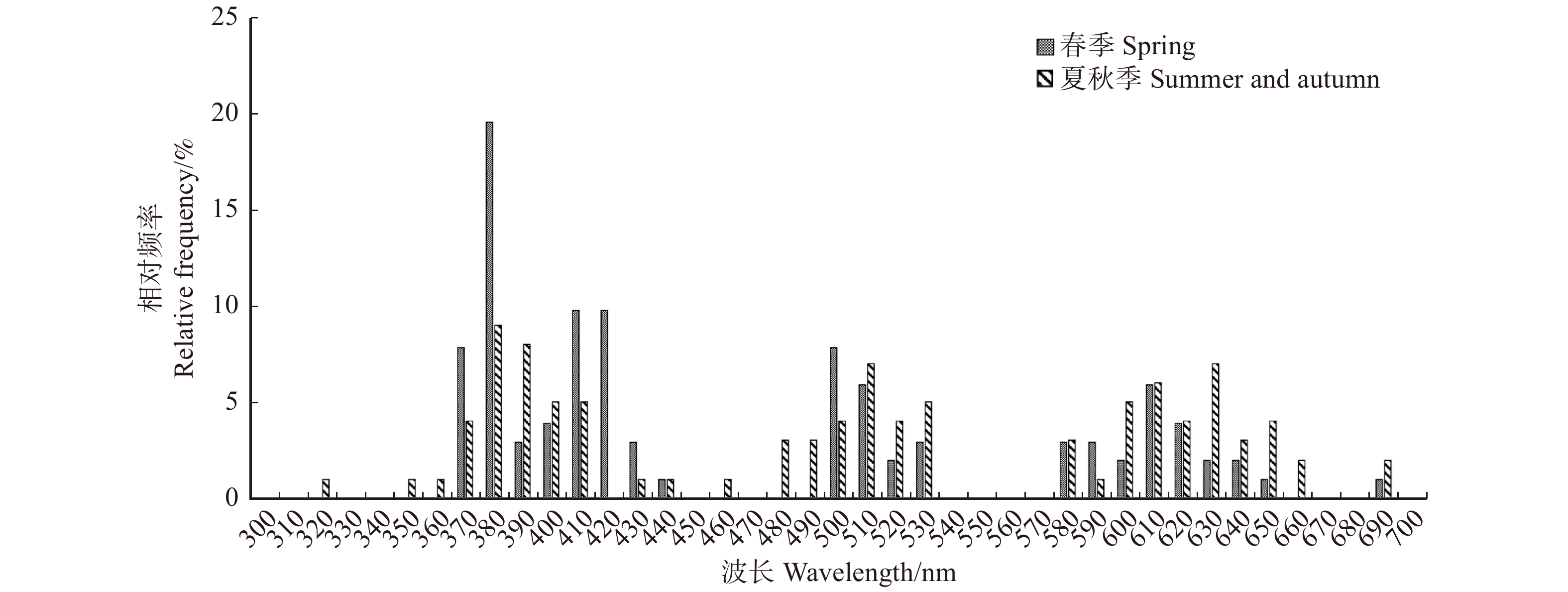
由图6可得,春季开花植物标记点多分布于紫光和蓝光波段(380 ~ 450 nm),标记点在380、510、620 nm波长(分别属于紫光、绿光和橙光波段)附近聚集形成3个密集分布峰;36.27%的标记点落在380 ~ 420 nm区间,13.73%的标记点分布于500 ~ 520 nm区间,13.73%的标记点分布于600 ~ 640 nm区间。夏秋季开花植物标记点分布较均匀,标记点在390、510 、630 nm波长(分别属于紫光、绿光和红光波段)附近聚集形成3个密集分布峰;27.00%的标记点分布于380 ~ 420 nm区间,11.00%的标记点分布于500 ~ 520 nm区间,22.00%的标记点分布于600 ~ 630 nm区间。
![]() 图 6 不同季节开花植物标记点分布频率Figure 6. Distribution frequency of flowering plant’s mark points in different seasons
图 6 不同季节开花植物标记点分布频率Figure 6. Distribution frequency of flowering plant’s mark points in different seasons不同季节开花植物的标记点MAD、minAD400、minAD500值如表1所示。春季开花植物的花色标记点MAD和minAD400显著低于夏秋季(P < 0.05),标记点minAD500不存在显著性差异,表明春季开花植物的花色光谱标记点与蜂类视觉敏感波段偏差距离相对较小,理论上比夏秋季开花植物更易被蜂类识别。
表 1 不同季节开花植物的标记点特征值Table 1. Characteristic values of mark-points of flowering plants in different seasons指标
Index春季
Spring夏秋季
Summer and autumnP MAD 47.23 ± 5.11 67.54 ± 5.72 0.012 minAD400 31.41 ± 7.95 84.63 ± 12.26 0.001 minAD500 59.86 ± 6.53 66.79 ± 6.89 0.478 注:MAD.平均绝对偏差;minAD.最小绝对偏差。下标400、500分别表示波长400、500 nm。Notes: MAD, mean absolute deviation; minAD, minimum absolute deviation. The subscripts 400 and 500 indicate wavelengths of 400 and 500 nm, respectively. 2.2.3 花色与背景的对比度分析
两个季节开花植物相对于背景的花色对比度特征存在明显差异(表2)。春季开花植物的非彩色对比度极显著高于夏秋季,春季开花植物的彩色对比度显著低于夏秋季。春季和夏秋季开花植物相对于背景的彩色对比度均值的差值未超过蜂类可辨别的最小差值。
表 2 不同季节开花植物的相对于背景的花色对比度特征值Table 2. Contrast against background values of flowering plants in different seasons指标
Index春季
Spring夏秋季
Summer and autumnP ACB 5.693 ± 2.664 2.858 ± 1.508 < 0.001 CCB 0.088 ± 0.052 0.115 ± 0.043 0.006 注:ACB.相对于背景的非彩色对比度;CCB.相对于背景的彩色对比度。Notes: ACB, achromatic contrast against the background; CCB, chromatic contrast against the background. 从蜂类视觉来看,以标准绿叶为背景时,春季开花植物与背景间的亮度差异和绿色反射率差异更大,夏秋季开花植物与背景间的色相差异和饱和度差异更大。
2.3 不同色系开花植物的花色分析
2.3.1 花色的标定与多样性分析
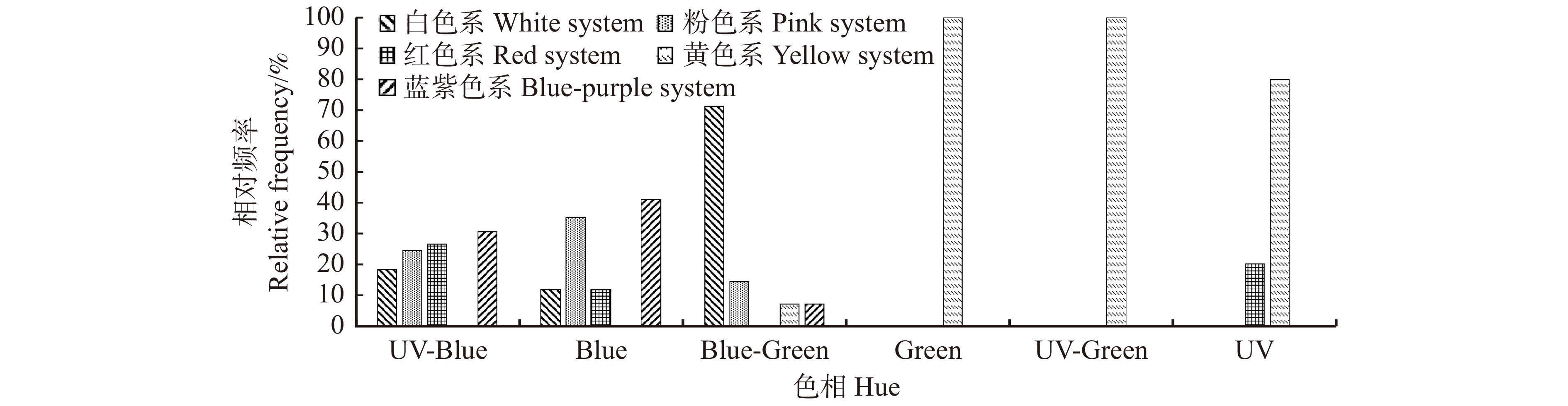
根据不同色系开花植物的色彩点位在CH模型中的位置,将其归为对应的色相并做统计(图7)。黄色系开花植物的花色标定后所包含蜂类视觉色相类型最多,即色相多样性最大,包括Blue-Green、Green、UV-Green和UV 4种色相,其中UV色相占比最高为42.11%,其次是Green(26.32%)、UV-Green(26.32%)、Blue-Green(5.26%)。经花色标定后,红色系开花植物所包括的蜂类视觉色相类型最少,仅有UV-Blue、Blue和UV 3种色相,其中UV-Blue色相占比最高为76.47%,Blue色相和UV色相占比均为11.76%。白色系、粉色系和蓝紫色系开花植物所包含的蜂类视觉色相类型均只有UV-Blue、Blue和Blue-Green 3种色相,白色系开花植物中这3种色相占比分别为42.86%、9.52%和47.62%,粉色系开花植物中这3种色相占比分别为60.00%、30.00%和10.00%,蓝紫系开花植中这3种色相占比分别为65.22%、30.43%和4.35%。
![]() 图 7 不同色系开花植物蜂类色相分布Figure 7. Hue distribution in the bees vision of flowering plants in different colors
图 7 不同色系开花植物蜂类色相分布Figure 7. Hue distribution in the bees vision of flowering plants in different colors蜂类视觉下的色相对应的开花植物色系分布如图8所示。蜂类视觉的色相与人类视觉的色相不存在明显的对应关系。各色相中,UV-Blue、Blue和Blue-Green色相所对应的花色较丰富,UV、Green和UV-Green色相所对应的花色较少。UV-Blue色相所对应的有蓝紫色系(30.61%)、红色系(26.53%)、粉色系(24.49%)、白色系(18.37%),Blue色相所对应的有蓝紫色系(41.18%)、粉色系(35.29%)、白色系(11.76%)和红色系(11.76%),Blue-Green色相所对应的有白色系(71.43%)、粉色系(14.29%)、黄色系(7.14%)和蓝紫色系(7.14%),UV色相所对应的有黄色系(80.00%)和红色系(20.00%)两种,Green和UV-Green色相均只对应黄色系。
![]() 图 8 不同蜂类色相开花植物色系分布Figure 8. Color distribution of flowering plants of different hues in bees vision
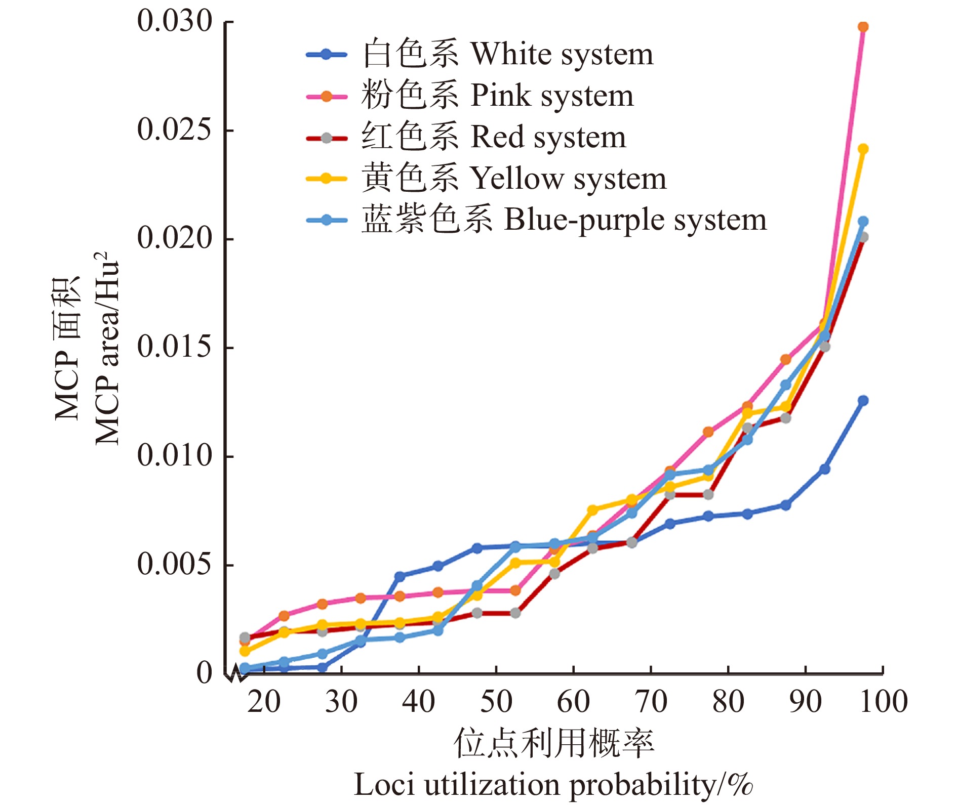
图 8 不同蜂类色相开花植物色系分布Figure 8. Color distribution of flowering plants of different hues in bees vision进一步比较花色多样性,计算不同色系开花植物的MCP面积(图9)。取点位利用率为85%和100%时的MCP面积进行分析,粉色系开花植物的MCP面积最大,其次是黄色系、蓝紫色系、红色系开花植物,白色系开花植物的MCP面积最小。由数据可得,粉色系开花植物和黄色系开花植物的花色多样性较大,说明属于粉色系的不同开花植物在蜂类视觉中差异较大,属于黄色系的不同开花植物在蜂类视觉中的差异也较大;而白色系开花植物的花色多样性较小,即属于白色系的不同开花植物在蜂类视觉中差异较小。
![]() 图 9 不同色系植物色彩位点MCP面积Figure 9. MCP area of color loci of flowering plants in different color systems
图 9 不同色系植物色彩位点MCP面积Figure 9. MCP area of color loci of flowering plants in different color systems2.3.2 标记点分布特征分析
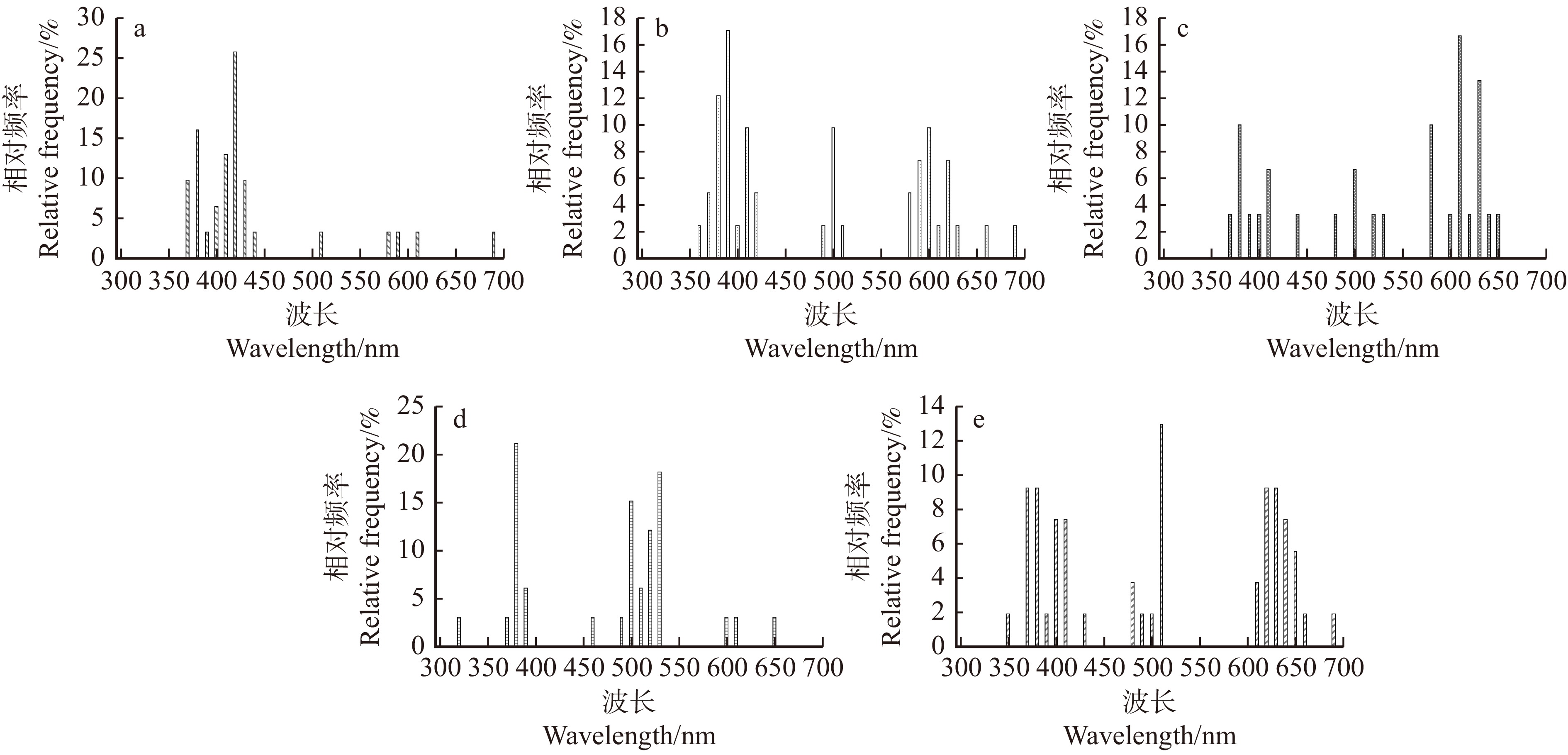
不同色系开花植物的标记点分布特征有一定差异(图10)。白色系开花植物的标记点多分布于紫光和蓝光波段(380 ~ 450 nm),主要在420 nm波长(属于紫光波段)附近形成一个密集分布峰。粉色系开花植物的标记点在390、500和600 nm波长(分别属于紫光、绿光和橙光波段)附近形成3个密集分布峰。红色系开花植物的标记点多分布于橙光和红光波段(590 ~ 660 nm),在390、500和620 nm波长(分别属于紫光、绿光和红光波段)附近形成3个密集分布峰。黄色系开花植物的标记多分布于绿光波段(490 ~ 540 nm),在380和500 nm波长(分别属于紫光和绿光波段)附近形成两个密集分布峰。蓝紫色系开花植物的标记点分布比较均匀,在380、500和620 nm波长(分别属于紫光、绿光和红光波段)附近形成3个密集分布峰。
![]() 图 10 不同色系开花植物标记点分布频率a.白色系开花植物;b.粉色系开花植物;c.红色系开花植物;d.黄色系开花植物;e.蓝紫色系开花植物。a, white flowering plants;b, pink flowering plants;c, red flowering plants;d, yellow flowering plants;e, blue-purple flowering plants.Figure 10. Distribution frequency of flowering plant’s mark points in different color systems
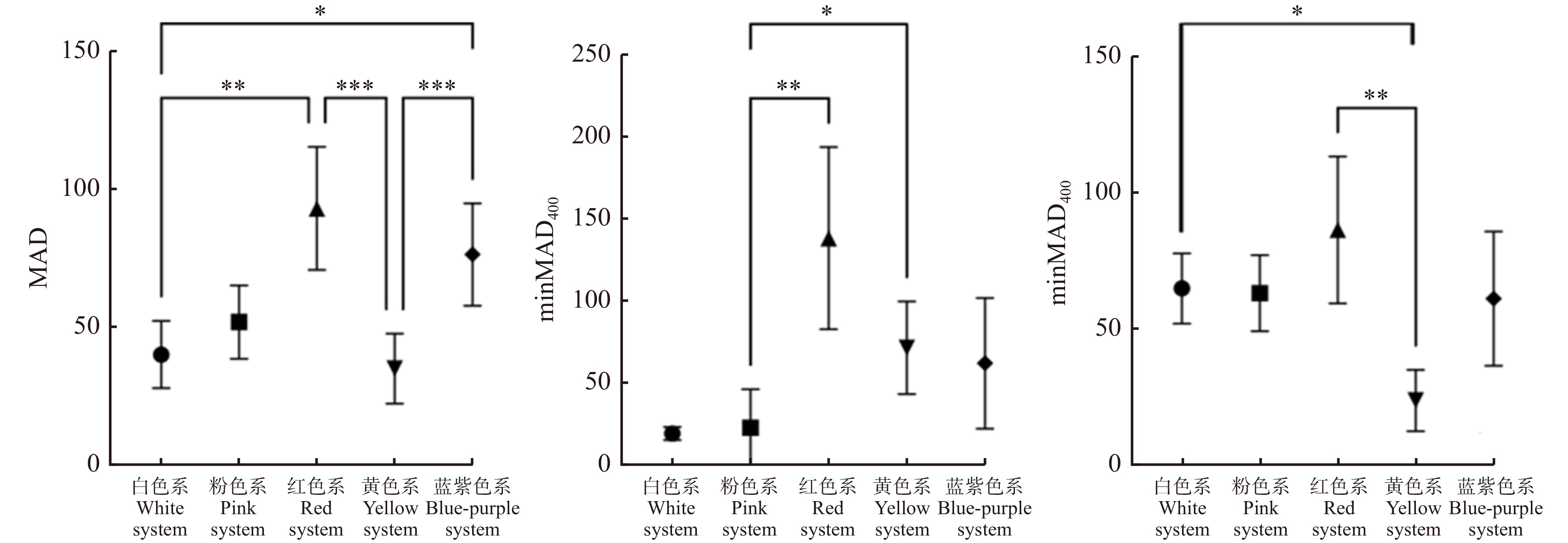
图 10 不同色系开花植物标记点分布频率a.白色系开花植物;b.粉色系开花植物;c.红色系开花植物;d.黄色系开花植物;e.蓝紫色系开花植物。a, white flowering plants;b, pink flowering plants;c, red flowering plants;d, yellow flowering plants;e, blue-purple flowering plants.Figure 10. Distribution frequency of flowering plant’s mark points in different color systems不同色系开花植物的花色标记点存在显著差异(PMAD < 0.001,PminAD400 = 0.002,PminAD500 = 0.009)。对于MAD,红色系开花植物的偏差值最大,其次是蓝紫色系、粉色系和白色系开花植物,黄色系开花植物的偏差值最小;红色系开花植物与白色系、黄色系开花植物的偏差值存在极显著差异,蓝紫色系开花植物与白色系开花植物的偏差值存在显著差异,蓝紫色系开花植物与黄色系开花植物的偏差值存在极显著差异。对于minAD400,红色系开花植物的偏差值最大,其次是黄色系、蓝紫色系开花植物,白色系和粉色系开花植物的偏差值较小;红色系开花植物与粉色系开花植物的偏差值存在极显著差异,黄色系开花植物与粉色系开花植物的偏差值存在显著差异。对于minAD500,红色系开花植物的偏差值最大,白色系、粉色系和蓝紫色系开花植物的偏差值相近,黄色系开花植物的偏差值最小;黄色系开花植物与红色系的偏差值存在极显著差异,与白色系开花植物的偏差值存在显著差异(图11)。
![]() 图 11 不同色系开花植物标记点分布特征值*.P < 0.05;**.P < 0.01;***.P < 0.001。下同。Same as below.Figure 11. Characteristic values of marker-points of flowering plants in different color systems
图 11 不同色系开花植物标记点分布特征值*.P < 0.05;**.P < 0.01;***.P < 0.001。下同。Same as below.Figure 11. Characteristic values of marker-points of flowering plants in different color systems2.3.3 花色与背景的对比度分析
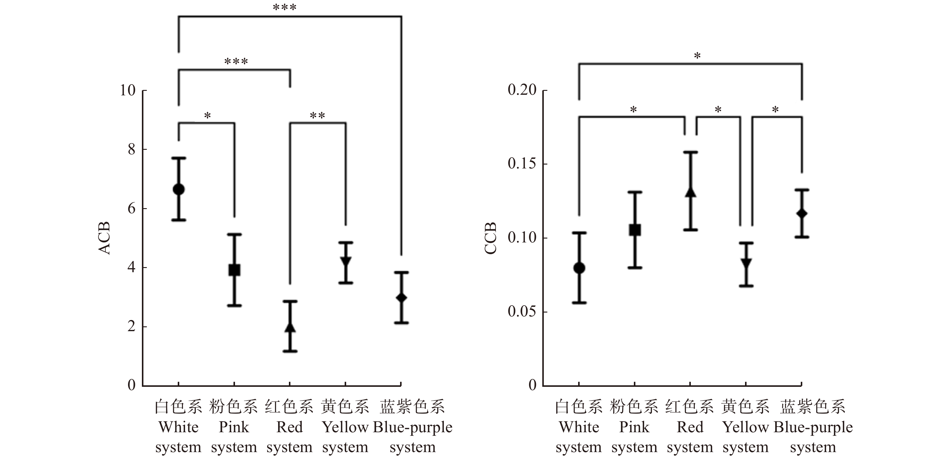
不同色系的开花植物的ACB与CCB值存在显著差异(PACB < 0.001,PCCB < 0.001)。对于ACB,白色系开花植物的非彩色对比度最大,其次是黄色系、粉色系和蓝紫色系开花植物,红色系开花植物的非彩色对比度最小;白色系开花植物与蓝紫色系、红色系开花植物的非彩色对比度存在极显著差异,白色系开花植物与粉色系开花植物的非彩色对比度存在显著差异,黄色系开花植物与红色系开花植物的非彩色对比度存在极显著差异。对于CCB,红色系开花植物的彩色对比度最大,其次是蓝紫色系和粉色系开花植物,白色系和黄色系开花植物的彩色对比度较小;白色系开花植物与红色系、蓝紫色系开花植物的彩色对比度存在显著差异,黄色系开花植物与红色系、蓝紫色系开花植物的彩色对比度存在显著差异(图12)。
![]() 图 12 不同色系开花植物相对于背景的花色对比度Figure 12. Contrast against background values of flowering plants in different color systems
图 12 不同色系开花植物相对于背景的花色对比度Figure 12. Contrast against background values of flowering plants in different color systems3. 结论与讨论
不同季节开花植物的花色多样性、标记点分布特征和花色与背景的对比度存在差异。在花色多样性方面,夏秋季开花植物的花色多样性更大,在蜂类视觉中颜色差异较大。在标记点分布特征方面,春季开花植物的标记点多分布于紫光和蓝光波段(380 ~ 450 nm),而夏秋季开花植物的标记点分布相对较均匀。春季开花植物的花色光谱标记点偏差值较小,理论上比夏秋季开花植物更易被蜂类识别。在花色与背景的对比度方面,春季开花植物的非彩色对比度大,可能与蜂类绿色光感受器所感知到的非彩色对比度有助于其在远距离搜寻开花植物有关[26]。推测春季开花植物较少,此类植物可利用该特点招引较远距离的蜂类昆虫;夏秋季开花植物的彩色对比度较大,原因可能是夏秋季的红色系开花植物明显多于春季。两个采样季开花植物的ACB和CCB特征不同,推测在不同的环境和背景下,两个采样季开花植物形成的以花色来招引蜂类的策略不同。有研究认为蜂类偏好UV-Blue色相[39],本研究发现两个季节的UV-Blue色相的植物均较多。此外,两个季节的开花植物的标记点均在390、510、620 nm波长附近聚集分布,符合蜂类在400 nm和500 nm附近有最高敏感度的特征,而长波处出现了标记点密集峰可能与植物组织的一般反射特性有关[33]。通过两个季节开花植物具有的相似花色特征可以推测出,北京公园常用园林植物具有一定的蜂类招引能力,可以为蜂类提供一定生境条件。总体而言,北京公园常用园林植物春季开花植物更易被蜂类感知,但花色多样性较低。而北京2月即可观察到蜂类访花行为,因此可以选育和应用更多的春花植物,可提高蜂类的取食效率。
不同色系开花植物的花色多样性、标记点分布特征和花色与背景的对比度存在差异。在花色多样性方面,黄色系开花植物包括最多的蜂类视觉色相,红色系开花植物包括最少的蜂类视觉色相,根据MCP值,黄色系和粉色系开花植物的花色多样性最大,红色系开花植物的花色多样性最小。在标记点分布特征方面,黄色系开花植物的minAD500较小,粉色系和白色系开花植物的minAD400较小,红色系开花植物的两个标记点偏差值均最大,黄色系、粉色系和白色系开花植物较易被蜂类识别,红色系开花植物较难被蜂类识别。在花色与背景的对比度方面,白色系开花植物的非彩色对比度最大,红色系开花植物的非彩色对比度最小,红色系开花植物的彩色对比度最大,黄色系开花植物的非彩色对比度最小。前人研究表明,蜂类对长波相对不敏感[47],较难分辨出红色花[48]。此外,红色花在复杂背景下更难被蜂类识别出来[49]。理论上红色系开花植物的ACB和CCB值均应较小,但是本研究计算出的红色花CCB值较大,可能与ACB和CCB在不同条件下对蜂类识别花有不同的作用效果有关:一是蜂类与目标物的距离,非彩色对比度是蜂类远距离识别花的信号,在蜂类进近飞行时,这种信号将先于彩色对比度被感应到[50];二是目标物的大小,当目标物较小时,欧洲熊蜂(Bombus terrestris)识别目标物的时间与非彩色对比度相关,而目标物较大时,识别时间与彩色对比度相关,蜜蜂对两种颜色花朵的相对偏好可能会根据花朵的大小而改变[51]。根据相关分析,在北京公园常用园林植物中,黄色系、白色系和粉色系开花植物理论上较易被蜂类感知,红色系开花植物较难被感知。
北京地区常见蜂类有意大利蜂(A. mellifera)、中华蜜蜂(A. cerana)和熊蜂属、地蜂属(Andrena)、淡脉隧蜂属(Lasioglossum)等。在温带地区,蜂群种群的年数量变化动态大体可分为春季增长、越夏下降、秋季增长和越冬下降4个阶段。北京地区的熊蜂一年一代,在早春植物开花时开始活动,到盛夏时蜂群达到最盛,蜂群继续活动至冬季气温降低,其主要传粉季在夏秋[52-53]。结合北京地区常见蜂类的种群动态和生活习性,本文以3—10月的开花植物为研究对象,植物花期与北京地区蜂类传粉活动的主要时间吻合。
若根据花色筛选蜂类招引类植物,可选择非彩色对比度、彩色对比度和花色光谱标记点偏差值作为标准。根据本研究的结果,在北京地区的常用园林植物中,八棱海棠(Malus robusta)、山杏(Prunus sibirica)、诸葛菜(Orychophragmus violaceus)、‘染井吉野’樱(P. × yedoensis ‘Somei-yoshino’)等非彩色对比度较高,白车轴草(Trifolium repens)、花毛茛(Ranunculus asiaticus)、紫茉莉(Mirabilis jalapa)、蓝花鼠尾草(Salvia farinacea)等彩色对比度较高,柳叶白菀(Aster ericoides)、黄刺玫(Rosa xanthina)、小菊‘绚秋莲华’(Chrysanthemum‘Xuanqiu Lianhua’)、小菊‘绚秋粉黛’(C. ‘Xuanqiu Fendai’)、迎春花(Jasminum nudiflorum)等标记点偏差值较小,以上植物理论上较易被蜂类识别,招引能力较强。在分类学上属同一目的昆虫光感受器特征相对比较固定[27],膜翅目昆虫的视觉系统与蜜蜂的视觉系统相似,具有相似的光谱敏感性函数的峰值位置。本研究基于蜂类三色光感受器敏感函数和CH模型的分析结果可以在一定程度上推广至整个膜翅目传粉昆虫[54]。
除花色外,花形、花香等视觉或嗅觉信号也可作为植物招引传粉昆虫的信号。花形易受环境影响,难以作为稳定性状进行蜂类友好型植物的筛选。对于花香而言,前人研究了小花矮牵牛属(Calibrachoa)品种的花香特征与访花昆虫(以蜂类为主)访花偏好之间的关系,只发现少数的单一化合物可能与传粉昆虫偏好相关[55]。本研究重点开展了花色特征对蜂类访花偏好的影响,未来将继续深入研究花形、花香等其他花部特征,以及植物群落组成与结构等对蜂类访花偏好的影响,综合评估开花植物对蜂类的招引能力,构建全面系统的传粉昆虫友好型园林植物筛选体系。
-
![]()
图 1 开花植物在波长300 ~ 700 nm的反射比
红色曲线为取中位数后的反射曲线,浅红色范围为标准偏差。The red curve is the reflection curve after taking the median, and the light red range represents the standard deviation.
Figure 1. Total reflectance at wavelength 300−700 nm of the flowering plants
![]()
图 2 开花植物在蜂类视觉颜色空间中的色彩位点
六边形的6个扇区分别表示不同的蜂类视觉颜色。EB、EG、EUV分别代表蓝色光、绿色光和紫外光感受器的相对刺激值。The six sectors of the hexagon represent different color types of bees version. EB, EG, EUV represent the relative stimulus values of blue light, green light, and UV receptors, respectively.
Figure 2. Color loci in bees space of the flowering plants
![]()
图 5 不同季节植物色彩位点MCP面积
MCP. 最小凸多边形。不同点位利用概率表示落在MCP内的色彩位点百分比,依次排除距离所有点位中心最远的点。MCP, minimum convex polygon. The point utilization probability represents the percentage of color loci in the MCP, and the points farthest from the centers of all points are excluded in turn.
Figure 5. MCP area of plant color loci in different seasons
![]()
图 6 不同季节开花植物标记点分布频率
Figure 6. Distribution frequency of flowering plant’s mark points in different seasons
![]()
图 7 不同色系开花植物蜂类色相分布
Figure 7. Hue distribution in the bees vision of flowering plants in different colors
![]()
图 8 不同蜂类色相开花植物色系分布
Figure 8. Color distribution of flowering plants of different hues in bees vision
![]()
图 9 不同色系植物色彩位点MCP面积
Figure 9. MCP area of color loci of flowering plants in different color systems
![]()
图 10 不同色系开花植物标记点分布频率
a.白色系开花植物;b.粉色系开花植物;c.红色系开花植物;d.黄色系开花植物;e.蓝紫色系开花植物。a, white flowering plants;b, pink flowering plants;c, red flowering plants;d, yellow flowering plants;e, blue-purple flowering plants.
Figure 10. Distribution frequency of flowering plant’s mark points in different color systems
![]()
图 11 不同色系开花植物标记点分布特征值
*.P < 0.05;**.P < 0.01;***.P < 0.001。下同。Same as below.
Figure 11. Characteristic values of marker-points of flowering plants in different color systems
![]()
图 12 不同色系开花植物相对于背景的花色对比度
Figure 12. Contrast against background values of flowering plants in different color systems
表 1 不同季节开花植物的标记点特征值
Table 1 Characteristic values of mark-points of flowering plants in different seasons
指标
Index春季
Spring夏秋季
Summer and autumnP MAD 47.23 ± 5.11 67.54 ± 5.72 0.012 minAD400 31.41 ± 7.95 84.63 ± 12.26 0.001 minAD500 59.86 ± 6.53 66.79 ± 6.89 0.478 注:MAD.平均绝对偏差;minAD.最小绝对偏差。下标400、500分别表示波长400、500 nm。Notes: MAD, mean absolute deviation; minAD, minimum absolute deviation. The subscripts 400 and 500 indicate wavelengths of 400 and 500 nm, respectively.  下载: 导出CSV
表 2 不同季节开花植物的相对于背景的花色对比度特征值
Table 2 Contrast against background values of flowering plants in different seasons
指标
Index春季
Spring夏秋季
Summer and autumnP ACB 5.693 ± 2.664 2.858 ± 1.508 < 0.001 CCB 0.088 ± 0.052 0.115 ± 0.043 0.006 注:ACB.相对于背景的非彩色对比度;CCB.相对于背景的彩色对比度。Notes: ACB, achromatic contrast against the background; CCB, chromatic contrast against the background.
下载: 导出CSV
-
[1] 袁嘉, 杜春兰. 城市植物景观与关键种的协同共生设计框架: 以野花草甸与传粉昆虫为例[J]. 风景园林, 2020, 27(4): 50−55. Yuan J, Du C L. Design framework of collaborative symbiosis between urban plant landscape and keystone species: taking wildflower meadows and pollinators as a case study[J]. Landscape Architecture, 2020, 27(4): 50−55.
[2] Jeff O. Pollinator diversity: Distribution, ecological function and conservation[J]. Annual Review of Ecology, Evolution, and Systematics, 2017, 48: 353−376. doi: 10.1146/annurev-ecolsys-110316-022919
[3] Potts S G, Imperatriz-Fonseca V, Ngo H T, et al. Safeguarding pollinators and their values to human well-being[J]. Nature, 2016, 540: 220−229. doi: 10.1038/nature20588
[4] 伍盘龙, 宋潇, 夏博辉, 等. 北京昌平区农业景观野生蜂多样性的时空动态分布[J]. 中国生态农业学报, 2018, 26(3): 357−366. Wu P L, Song X, Xia B H, et al. Temporal-spatial dynamics of wild bee diversity in agricultural landscapes in Changping District, Beijing[J]. Chinese Journal of Eco-Agriculture, 2018, 26(3): 357−366.
[5] van der Kooi C J, Dyer A, Kevan P G, et al. Functional significance of the optical properties of flowers for visual signalling[J]. Annals of Botany, 2019, 123(2): 263−276. doi: 10.1093/aob/mcy119
[6] Fenster C B, Armbruster W S, Wilson P, et al. Pollination syndromes and floral specialization[J]. Annual Review of Ecology, Evolution, and Systematics, 2004, 35(1): 375−403. doi: 10.1146/annurev.ecolsys.34.011802.132347
[7] Raguso R A. Flowers as sensory billboards: progress towards an integrated understanding of floral[J]. Current Opinion in Plant Biology, 2004, 7(4): 434−440. doi: 10.1016/j.pbi.2004.05.010
[8] Schäffler I, Steiner K E, Haid M, et al. Diacetin, a reliable cue and private communication channel in a specialized pollination system[J/OL]. Scientific Reports, 2015, 5: 12779[2022−01−18]. https://www.nature.com/articles/srep12779.
[9] Raguso R A. Wake up and smell the roses: the ecology and evolution of floral scent[J]. Annual Review of Ecology, Evolution, and Systematics, 2008, 39(1): 549−569. doi: 10.1146/annurev.ecolsys.38.091206.095601
[10] Yoshida M, Itoh Y, Ômura H, et al. Plant scents modify innate colour preference in foraging swallowtail butterflies[J/OL]. Biology Letters, 2015, 11(7): 20150390[2022−01−18]. https://royalsocietypublishing.org/doi/10.1098/rsbl.2015.0390.
[11] Woodcock T S, Larson B M H, Kevan P G, et al. Flies and flowers Ⅱ: floral attractants and rewards[J]. Journal of Pollination Ecology, 2014, 12: 63−94. doi: 10.26786/1920-7603(2014)5
[12] Lázaro A, Hegland S J, Totland Ø. The relationships between floral traits and specificity of pollination systems in three Scandinavian plant communities[J]. Oecologia, 2008, 157(2): 249−257. doi: 10.1007/s00442-008-1066-2
[13] Arnold S E J, Chittka L. Flower colour diversity seen through the eyes of pollinators. A commentary on: ‘floral colour structure in two Australian herbaceous communities: it depends on who is looking’[J]. Annals of Botany, 2019, 124(2): 8−9.
[14] Ohashi K, Makino T T, Arikawa K. Floral colour change in the eyes of pollinators: testing possible constraints and correlated evolution[J]. Functional Ecology, 2015, 29(9): 1144−1155. doi: 10.1111/1365-2435.12420
[15] Dyer A G, Boyd-Gerny S, Shrestha M, et al. Innate colour preferences of the Australian native stingless bee Tetragonula carbonaria Sm.[J]. Journal of Comparative Physiology A, 2016, 202: 603−613. doi: 10.1007/s00359-016-1101-4
[16] Erickson E, Adam S, Russo L, et al. More than meets the eye? The role of annual ornamental flowers in supporting pollinators[J]. Environmental Entomology, 2020, 49(1): 178−188. doi: 10.1093/ee/nvz133
[17] Kinoshita M, Takahashi Y, Arikawa K. Simultaneous brightness contrast of foraging Papilio butterflies[J]. Proceedings of the Royal Society B: Biological Sciences, 2012, 279: 1911−1918. doi: 10.1098/rspb.2011.2396
[18] Lunau K, Maier E J. Innate colour preferences of flower visitors[J]. Journal of Comparative Physiology A, 1995, 177(1): 1−19.
[19] Dyer A G, Boyd-Gerny S, Shrestha M, et al. Colour preferences of Tetragonula carbonaria Sm. stingless bees for colour morphs of the Australian native orchid Caladenia carnea[J]. Journal of Comparative Physiology A, 2019, 205(3): 347−361. doi: 10.1007/s00359-019-01346-0
[20] Waser N M, Price M V. Pollinator behaviour and natural selection for flower colour in Delphinium nelsonii[J]. Nature, 1983, 302: 422−424. doi: 10.1038/302422a0
[21] Shrestha M, Dyer A G, Bhattarai P, et al. Flower colour and phylogeny along an altitudinal gradient in the Himalayas of Nepal[J]. Journal of Ecology, 2014, 102(1): 126−135. doi: 10.1111/1365-2745.12185
[22] de Jager M L, Dreyer L L, Ellis A G. Do pollinators influence the assembly of flower colours within plant communities?[J]. Oecologia, 2011, 166(2): 543−553. doi: 10.1007/s00442-010-1879-7
[23] Shrestha M, Garcia J E, Martin B, et al. Australian native flower colours: does nectar reward drive bee pollinator flower preferences?[J/OL]. PLoS ONE, 2020, 15(6): e226469[2021−01−11]. https://journals.plos.org/plosone/article?id=10.1371/journal.pone.0226469.
[24] Lunau K, Papiorek S, Eltz T, et al. Avoidance of achromatic colours by bees provides a private niche for hummingbirds[J]. Journal of Experimental Biology, 2011, 214(9): 1607−1612. doi: 10.1242/jeb.052688
[25] 杨丽莉. 青藏高原高寒草地植物群落花色多样性及影响因素[D]. 兰州: 兰州大学, 2020. Yang L L. Flower color diversity and influencing factors in alpine meadow community of Qinghai-Tibet Plateau[D]. Lanzhou: Lanzhou University, 2020.
[26] Gray M, Stansberry M J, Lynn J S, et al. Consistent shifts in pollinator-relevant floral coloration along Rocky Mountain elevation gradients[J]. Journal of Ecology, 2018, 106(5): 1910−1924. doi: 10.1111/1365-2745.12948
[27] Chittka L. The colour hexagon: a chromaticity diagram based on photoreceptor excitations as a generalized representation of colour opponency[J]. Journal of Comparative Physiology A, 1992, 170(5): 533−543.
[28] 李庆良, 马晓开, 程瑾, 等. 花颜色和花气味的量化研究方法[J]. 生物多样性, 2012, 20(3): 308−316. Li Q L, Ma X K, Cheng J, et al. Quantitative studies of floral color and floral scent[J]. Biodiversity Science, 2012, 20(3): 308−316.
[29] Shrestha M, Dyer A G, Burda M. Evaluating the spectral discrimination capabilities of different pollinators and their effect on the evolution of flower colors[J/OL]. Communicative & Integrative Biology, 2013, 6(3): e24000−1−4[2021−04−23]. https://www.tandfonline.com/action/showCitFormats?doi=10.4161%2Fcib.24000.
[30] Tai K C, Shrestha M, Dyer A G, et al. Floral color diversity: how are signals shaped by elevational gradient on the tropical-subtropical mountainous island of Taiwan?[J/OL]. Frontiers in Plant Science, 2020, 11: 582784[2021−02−10]. https://www.frontiersin.org/articles/10.3389/fpls.2020.582784/full.
[31] Shrestha M, Dyer A G, Boyd G S, et al. Shades of red: bird-pollinated flowers target the specific colour discrimination abilities of avian vision[J]. The New phytologist, 2013, 198(1): 301−310. doi: 10.1111/nph.12135
[32] Dyer A G, Boyd-Gerny S, McLoughlin S, et al. Parallel evolution of angiosperm colour signals: common evolutionary pressures linked to hymenopteran vision[J]. Proceedings of the Royal Society B:Biological Sciences, 2012, 279(1742): 3606−3615. doi: 10.1098/rspb.2012.0827
[33] Camargo M G G, Cazetta E, Schaefer H M, et al. Fruit color and contrast in seasonal habitats: a case study from a cerrado savanna[J]. Oikos, 2013, 122(9): 1335−1342. doi: 10.1111/j.1600-0706.2013.00328.x
[34] Camargo M G G, Lunau K, Batalha M A, et al. How flower colour signals allure bees and hummingbirds: a community-level test of the bee avoidance hypothesis[J]. The New phytologist, 2019, 222(2): 1112−1122. doi: 10.1111/nph.15594
[35] Shrestha M, Lunau K, Dorin A, et al. Floral colours in a world without birds and bees: the plants of Macquarie Island[J]. Plant Biology (Stuttgart, Germany), 2016, 18(5): 842−850. doi: 10.1111/plb.12456
[36] Tunes P, Camargo M G G, Guimarães E. Floral UV features of plant species from a neotropical savanna[J/OL]. Frontiers in Plant Science, 2021, 12: 618028[2022−01−10]. https://www.frontiersin.org/articles/10.3389/fpls.2021.618028/full.
[37] Dorin A, Shrestha M, Herrmann M, et al. Automated calculation of spectral-reflectance marker-points to enable analysis of plant colour-signalling to pollinators[J/OL]. MethodsX, 2020, 7: 100827[2021−03−21]. https://www.sciencedirect.com/science/article/pii/S2215016120300479?via%3Dihub.
[38] Papiorek S, Junker R R, Alves-Dos-Santos I, et al. Bees, birds and yellow flowers: pollinator-dependent convergent evolution of UV patterns[J]. Plant Biology, 2016, 18(1): 46−55. doi: 10.1111/plb.12322
[39] Giurfa M, Núnez J, Chittka L, et al. Colour preferences of flower-naive honeybees[J]. Journal of Comparative Physiology A, 1995, 177(3): 247−259.
[40] Koethe S, Bossems J, Dyer A G, et al. Colour is more than hue: preferences for compiled colour traits in the stingless bees Melipona mondury and M. quadrifasciata[J]. Journal of Comparative Physiology A, 2016, 202(9−10): 615−627. doi: 10.1007/s00359-016-1115-y
[41] Aguiar J M R B, Maciel A A, Santana P C, et al. Intrafloral color modularity in a bee-pollinated orchid[J/OL]. Frontiers in Plant Science, 2020, 11: 589300[2021−01−11]. https://www.frontiersin.org/articles/10.3389/fpls.2020.589300/full.
[42] Dalrymple R L, Kemp D J, Flores-Moreno H, et al. Macroecological patterns in flower colour are shaped by both biotic and abiotic factors[J]. New Phytologist, 2020, 228(6): 1972−1985. doi: 10.1111/nph.16737
[43] Streinzer M, Neumayer J, Spaethe J. Flower color as predictor for nectar reward quantity in an alpine flower community[J/OL]. Frontiers in Ecology and Evolution, 2021, 9: 721241[2022−01−05]. https://www.frontiersin.org/articles/10.3389/fevo.2021.721241/full.
[44] Bergamo P J, Telles F J, Arnold S E J, et al. Flower colour within communities shifts from over dispersed to clustered along an alpine altitudinal gradient[J]. Oecologia, 2018, 188(1): 223−235. doi: 10.1007/s00442-018-4204-5
[45] Bukovac Z, Shrestha M, Garcia J E, et al. Why background colour matters to bees and flowers[J]. Journal of Comparative Physiology A, 2017, 203(5): 369−380. doi: 10.1007/s00359-017-1175-7
[46] Martins A E, Arista M, Morellato L P C, et al. Color signals of bee-pollinated flowers: the significance of natural leaf background[J]. American Journal of Botany, 2021, 108(5): 788−797. doi: 10.1002/ajb2.1656
[47] Proctor M C F, Yeo P, Lack A. The natural history of pollination[M]. London: Harper Collins Publishers, 1996.
[48] Chittka L, Waser N M. Why red flowers are not invisible to bees[J]. Israel Journal of Plant Sciences, 1997, 45(2−3): 169−183. doi: 10.1080/07929978.1997.10676682
[49] Forrest J, Thomson J D. Background complexity affects colour preference in bumblebees[J]. Naturwissenschaften, 2009, 96(8): 921−925. doi: 10.1007/s00114-009-0549-2
[50] Giurfa M, Vorobyev M, Kevan P, et al. Detection of coloured stimuli by honeybees: minimum visual angles and receptor specific contrasts[J]. Journal of Comparative Physiology A, 1996, 178(5): 699−709.
[51] Spaethe J, Tautz J, Chittka L. Visual constraints in foraging bumblebees: flower size and color affect search time and flight behavior[J]. Proceedings of the National Academy of Sciences of the United States of America, 2001, 98(7): 3898−3903. doi: 10.1073/pnas.071053098
[52] 黄家兴. 华北地区熊蜂属(Hymenoptera: Apidae)系统发育的初步研究[D]. 北京: 中国农业科学院, 2006. Huang J X. The phylogeny of genus Bombus (Hymenopera: Apidae) in North China[D]. Beijing: Chinese Academy of Agricultural Sciences, 2006.
[53] 彭文君, 黄家兴, 吴杰, 等. 华北地区六种熊蜂的地理分布及生态习性[J]. 昆虫知识, 2009, 46(1): 115−120. Peng W J, Huang J X, Wu J, et al. Geographic distribution and bionomics of six bumblebee species in North China[J]. Chinese Bulletin of Entomology, 2009, 46(1): 115−120.
[54] de Ibarra N H, Vorobyev M, Menzel R, et al. Mechanisms, functions and ecology of colour vision in the honeybee[J]. Journal of Comparative Physiology A, 2014, 200(6): 411−433. doi: 10.1007/s00359-014-0915-1
[55] Marquardt M, Kienbaum L, Losert D, et al. Comparison of floral traits in Calibrachoa cultivars and assessment of their impacts on attractiveness to flower-visiting insects[J]. Arthropod-Plant Interactions, 2021, 15(4): 517−534. doi: 10.1007/s11829-021-09844-2
-
期刊类型引用(13)
1. 夏甜甜,杜秋硕,刘鹏. 基于数字赋能的泰山古柏生态修复技术应用探究. 山东林业科技. 2024(02): 77-83 .  百度学术
百度学术
2. 叶程浩,杜晓晨,鲍宇. 一种基于YOLOv5和轮廓约束的木材空洞缺陷应力波层析成像算法. 木材科学与技术. 2023(05): 61-68 . 百度学术
3. 侯艳芳,王鑫,侯婷婷,郭靖,张艳. 古建筑木结构损伤检测方法研究进展. 粘接. 2022(01): 123-126+130 . 百度学术
4. 宋辉,姬晓文,高琦,缑鹏超,王志强. 基于数据驱动的不规则用电检测误差校正系统设计. 电子设计工程. 2022(06): 109-112+117 . 百度学术
5. 杨露露,董喜斌,徐华东. 电阻法和应力波法在活立木内部腐朽缺陷检测中的对比. 森林工程. 2022(04): 82-88 . 百度学术
6. 戴禄君,吴瑞瑞. 数据驱动的非线性光学显微成像误差校正研究. 激光杂志. 2022(07): 159-163 . 百度学术
7. 路程琳,何宇航,谢雨宏,刘依萍,刘嘉仪,王正. 应力波断层扫描法在立木检测方面的研究现状. 林业机械与木工设备. 2022(10): 37-40 . 百度学术
8. 刘涛,李光辉. 基于射线分割的林木应力波断层成像算法. 林业科学. 2021(09): 181-192 . 百度学术
9. 赵松,王勐. 移动AR+VR支持下全景图像拼接均匀性校正方法. 计算机仿真. 2021(11): 189-192+398 . 百度学术
10. 何宇航,陈偲,王弘历,黄席阳,王正. 断层扫描法在木材无损检测的研究进展. 木工机床. 2020(01): 13-16 . 百度学术
11. 张慧娟. 木材应力波检测精度的影响因素研究. 中国林副特产. 2020(01): 27-30 . 百度学术
12. 魏喜雯,孙丽萍,许述正,杨扬,杜春晓. 基于应力波传播速度模型的原木缺陷定量检测. 北京林业大学学报. 2020(05): 143-154 . 本站查看
13. 刘嘉新,高景泉,李超. 应用兰德韦伯算法的木材缺陷图像重建. 东北林业大学学报. 2019(12): 125-128 . 百度学术
其他类型引用(8)


计量
- 文章访问数: 561
- HTML全文浏览量: 168
- PDF下载量: 84
- 被引次数: 21
