
Comparison of methods for dividing developmental stages of natural mixed forest stands
-
摘要:目的
以长白山云冷杉针叶混交林为例,比较林分不同发育阶段划分的方法,确定最适宜长白山云冷杉针叶混交林发育阶段划分的方法,以便有针对性地制定不同发育阶段的森林经营策略,为天然林发育阶段的科学划分提供方法依据。
方法以吉林省汪清林业局金沟岭林场天然云冷杉针叶混交林为研究对象,共收集
2 589 个样地样本,采用种间联结−最优分割法(A)、林相特征判别法(B)、TWINSPAN双向指示物种分析法(C)、MRT多元回归树法(D)和基于TWINSPAN的判别分析法(E)5种方法,对云冷杉针叶混交林发育阶段进行划分。通过多重比较检验,验证不同发育阶段间是否存在显著差异,并使用吻合系数来评估不同方法划分结果间的一致性。最后,从树种组成和林分特征(包括样地的平均胸径、平均树高、公顷蓄积量、公顷株数、公顷生物量、公顷断面积、针阔比、物种多样性和径级大小多样性9个指标)方面,对5种方法的划分结果进行比较分析。结果多重比较的结果显示,用于描述林分特征的9个指标在不同发育阶段间基本存在显著差异,这表示结果较为可靠。方法D和方法E的吻合系数较高,表示这两种方法的划分结果较为一致;而方法B与其他方法的吻合性均较低。从林分的发育趋势来看,5种方法的划分结果大致相同。随着林分的逐渐发育,林分特征指标普遍增大,多样性指标降低,树种组成趋于简单。主要区别体现在公顷株数和树种组成指标,并且在不同方法的划分结果中,各个阶段之间指标的差异程度和每个阶段的样本量也有所不同。方法E的划分结果更符合林分的生长发育规律。具体来说,第1阶段云冷杉针叶混交林形成期,林分迅速生长;第2阶段林木间竞争加强期,个体显著分化;第3阶段林分发展为近自然林状态,即达到森林经营的目标状态。
结论基于TWINSPAN的判别分析法能更好地划分林分的发育阶段,并将长白山云冷杉针叶混交林的发育过程划分为建群阶段—竞争阶段—近自然林阶段,为森林的科学经营提供了重要理论依据。
Abstract:ObjectiveTaking the Changbai Mountain spruce coniferous mixed forest as an example, this study compared the methods for dividing different stages of forest development and determined the most suitable method for dividing the development stages of Changbai Mountain spruce coniferous mixed forest, aiming to develop targeted forest management strategies for different stages of development and provide a methodological basis for the scientific division of natural forest development stages.
MethodA total of
2 589 plot samples were divided by interspecies linkage-optimal segmentation method (A), forest facies characteristic discrimination method (B), TWINSPAN bidirectional indicator species analysis method (C), MRT multiple regression tree method (D), and TWINSPAN-based discriminant analysis method (E) of Jingouling Forest Farm of Wangqing Forestry Bureau of Jilin Province, northeastern China. Multiple comparisons were used to verify whether there were significant differences between different stages of stand development, and the anastomosis coefficient was used to compare the anastomosis between the classification results of different methods, and finally the classification results of five methods were compared from the aspects of tree species composition and stand characteristics.ResultThe results of multiple comparisons showed that the nine numerical indicators used to describe the characteristics of forest stands in this paper basically had significant differences between different stages of stand development, indicating that the results were more reliable. Method D and E had the highest anastomosis coefficient, indicating that the division results were more consistent, while method B had a low agreement with other methods. From the perspective of development trend of the stand, the results of each method are roughly the same. As the forest gradually developed, the forest characteristic indicators increased, the diversity indicators decreased, and the tree species composition tended to be simpler. The differences were mainly reflected in the number of hectares and tree species composition indicators, and in the division results of different methods, the degree of difference between the indicators and the sample size of each stage were also different. From the specific analysis of various aspects, the division results of method E were more in line with the growth and development law of stands. In the first stage, a mixed spruce and fir coniferous forest was formed, and the forest grew rapidly. In the second stage, competition between trees intensified, and individual differentiation was significant. In the third stage, the forest was classified as a near natural forest, which was the target state of forest management.
ConclusionThe discriminant analysis method based on TWINSPAN can better divide the developmental stage of forest stands, and divide the development process of Changbai Mountain spruce-fir-coniferous mixed forest into group establishment stage, competition stage and near-natural forest stage, which provides an important theoretical basis for forest scientific management.
-
以木结构为主的古建筑是我国的瑰宝,具有很高的历史、文化和艺术价值。然而由于木材本身的性质以及外界因素的影响,长期处在自然环境下的古建筑木结构会受到不同类型和程度的损伤,严重影响结构的安全性和稳定性。因此,为了实现对古建筑木结构的预防性保护[1],首先需要掌握构件的力学性能时变规律,然后对一定环境下构件的残余强度和剩余寿命等功能函数进行分析,最后跨越到以安全性为主的结构服役状态的评估。自19世纪四五十年代以来,研究人员就对木材强度随时间变化的规律展开研究。在得到木材强度受长期荷载作用随时间衰减的经验曲线的基础上,Gerhards等[2-3]基于累积损伤概念建立了长期荷载下木构件强度模型。考虑影响木构件承载力的其他因素,又分别建立了不同残损影响下的木构件损伤时变模型:李铁英[4]对中国古建筑木结构中的腐朽数据进行分析和整理,研究得到木构件腐朽层厚度随时间变化的发展规律,国内关于腐朽对木构件力学性能影响的众多研究均以此为分析基础;谢启芳等[5]通过去除腐朽部分来模拟木柱的局部残损,基于轴压试验和有限元模拟来分析局部损伤木柱的受力性能退化规律。考虑木材虫蛀,澳大利亚的CSIRO团队[6]根据现场调研获得的大量数据,建立了白蚁攻击木构件的风险演化模型,瞿伟廉等[7]基于该模型提出了理想环境下木材虫蛀与时间的数学模型,并据此推导出木构件的抗力衰减模型。而在木材干裂方面,基于对木材试验数据的拟合分析,彭磊等[8]提出了木构件开裂深度和含水率之间的变化关系;陈孔阳[9]通过力学试验、有限元数值模拟和理论分析,提出考虑纵向裂缝影响的梁、柱承载力计算公式;谢启芳等[10]对不同干裂程度的木柱进行轴压试验,考虑稳定系数、截面面积损失和初始偏心距3个影响参数,建立了自然干裂木柱的受压承载力和刚度退化模型。综合考虑多因素,王雪亮[11]和秦术杰[12]建立了受长期荷载、虫蛀、腐朽和干缩裂缝共同影响的木构件强度退化随机时变模型。由上所述,国内外对残损木构件强度退化的研究多针对单个影响因素,综合考虑多因素的较少。
同时,影响构件残损的因素,如环境温湿度、构件所用材种材性、荷载大小、承载面积等均具有随机不确定性,仅用“安全”或“失效”来评定其服役状态是不合理的,基于可靠度理论对木构件进行安全性评估是较为科学的分析方法。可靠度分析的传统算法有一次二阶矩法、二次二阶矩法、蒙特卡罗法和响应面法等[13]。对传统算法进行改进和结合,又衍化出适应不同情况的新算法。蒙特卡罗法(Monte Carlo method,MC)是可靠度分析较为常用的方法,但在参数较多的情况下,计算效率低,且不能保证结果的收敛性。近年来,针对随机结构动力系统分析,李杰等[14]基于有限单元法基本原理提出了概率密度演化方法(probability density evolution method,PDEM),弥补了传统可靠度算法存在的不足,在多个领域得到广泛应用,为可靠性分析开辟了新的道路。
如前所述,古建筑木构件的损伤是多因素综合作用的结果,需要考虑影响因素的随机性进行可靠度分析。因此,本研究考虑多种损伤,参考已有的单因子损伤时变模型建立木构件多因子损伤时变模型,并推导木构件强度退化模型;同时以一古建筑木结构的典型柱为例,基于概率密度演化方法对柱的残余强度进行可靠度分析,与蒙特卡罗法的分析结果进行对比,验证概率密度演化方法用于残损木构件可靠度分析的可行性。具体技术路线如图1所示。
1. 古建筑残损木构件强度退化时变模型
古建筑木构件在多因素的共同影响下产生损伤,而长期荷载、腐朽、虫蛀和干缩裂缝是对木构件力学性能影响较大的损伤[12],本章将基于前人研究建立的单因子损伤时变模型,构建综合考虑这4种残损的多因子损伤时变模型及强度退化模型。
1.1 单因子损伤时变模型
本节分别列出了仅考虑单一因素的木构件损伤时变模型,得到各因素影响下构件剩余有效截面积的时变模型,可作为构建多因子损伤时变模型的基础。
1.1.1 长期荷载
以Gerhards提出的累积损伤模型[2]为基础,推得木材强度随时间变化的预测模型[15]。
φM(t)=f(t)f0=1B2ln(1+(1−α(t))(expB2−1))=1B2ln(1+(1−exp(−B1+B2σf0))(expB2−1)) (1) 式中:
φM 为构件残余强度比,t为服役时间(a),f为长期荷载下木材的残余强度(MPa),f0 为短期静强度(MPa),α(t) 为随时间变化残余寿命的损伤率,其取值范围为[0,1],α(t)=0 时为无损状态,α(t)=1 时完全失效;σ 为外力作用下截面的最大应力(MPa),B1 、B2 为参数,需要通过试验进行标定。由式可知木材残余强度比是短期强度f0 、应力比σf0 和时间t的函数。1.1.2 腐 朽
根据李铁英总结出的古建筑木构件腐朽层厚度估计式[4],得到腐朽影响下构件截面积随时间变化率的估计式。
ξ(t)=(1−δ0d(1+T0t)α)2 (2) 式中:
ξ 为木构件的截面积变化率,δ0 为构件当前腐朽层厚度(mm),d为构件截面直径或边长(mm),T0 为预期已服役时间(a),t为时间(a),α 为考虑腐朽层厚度发展速度的指数参数:当t⩽400 时,α=1 ;当400<t⩽800 时,α=1.5 ;当t>800 ,暂无数据。构件截面积变化率是木构件当前腐朽层厚度δ0 与截面直径(或边长)d之比、预期服役时间T0 和时间t的函数。1.1.3 虫 蛀
基于CSIRO团队建立的随机虫蛀模型[6],将虫蛀过程分为初始期
tlag 和发展期td 两个阶段,得到虫洞引起构件的截面积损伤变量[16]。Dinsect(t)=a+bt (3) a=−btlag (4) 式中,
Dinsect(t) 为虫蛀引起的截面积损伤变量;a为建筑开始被虫蛀的时间(a);b为系数;tlag 为虫蛀初始期总时间(a),包括在建筑50 m范围内建立一个成熟蚁巢的时间t1 (a);白蚁形成虫道并到达建筑的时间t2 (a);白蚁突破或绕开所设置防蚁屏障的时间t3 (a),分别通过专家对各阶段内影响虫蛀事件的评估以及环境的优劣综合计算得到。1.1.4 干缩裂缝
假设裂缝均为图2所示的张开TR型[17]规则三角形裂缝,基于木构件相对开裂深度的时变模型[11,18]以及损伤变量的定义,得到受干缩裂缝影响有效截面积随时间变化的预测模型。
![]()
当木柱截面为圆形,则
Dcrack(t)=2λπ(exp(E+Fexp(kt)))2 (5) 当木柱截面为方形,则
Dcrack(t)=λ2(exp(E+Fexp(kt)))2 (6) 式中:
Dcrack(t) 为干缩开裂引起的截面积损伤变量,是随含水率和时间变化的函数。λ 为裂缝相对宽度和相对深度的比值,其取值范围一般为λ∈[0.15,0.25] [12];E 、F 为简化系数, E = C1 + C2CMC,F = C1C2CMC;C1、C2、k为参数,需通过试验标定;CMC 为相对平衡状态下的含水率。1.2 多因子强度退化模型
由上述单因子模型的分析可知,在各种因素的共同作用下,损伤累积使得构件有效截面积减小,应力随之发生变化。因此,基于累积损伤理论[2],通过逐年累加得到多因素作用下古建筑木结构残损构件的残余寿命损伤率随时间变化的关系式。
α(t)=∑ti=0exp(−B1+B2τ(i)) (7) 式中:
τ(i) 为木柱服役第i年时的应力比σ(i)f0 。此外,本节所有公式各参数含义均与上节相同。本文以古建筑木结构中柱的抗压强度退化为例,假设各影响因素相互独立,且受损伤部份完全失效,综合以上单因子模型,对考虑长期荷载、腐朽、虫蛀、干缩裂缝的残损木柱损伤时变模型及强度退化模型进行推导。
假设木柱(图3)轴心受压,在顺纹方向承受轴向压力N (N),服役初期初始截面积为
A0 (mm2),在服役时间为t年时有效截面积的值为A(t) (mm2)。根据上文所构建腐朽影响木构件剩余有效横截面积的时变模型(式(2))和虫蛀、干缩裂缝影响木构件有效截面积损伤变量的时变模型(式(3) ~ (6)),叠加3种类型的损伤,得到木柱有效截面积A随时间变化的模型。
A(t)=ξ(t)A0−Dinsect(t)A0−Dcrack(t)A0=(ξ(t)−Dinsect(t)−Dcrack(t))A0 (8) 则木柱有效截面积随时间的变化率
φ(t) 为φ(t)=ξ(t)−Dinsect(t)−Dcrack(t) (9) 由以上推导得到木柱在竖向荷载N作用下截面正应力
σ(t) 。σ(t)=NA(t)=Nφ(t)A0=σ0φ(t) (10) 式中:
σ0 为构件的初始应力(MPa)。木柱服役t年时应力比
τ(t) 为τ(t)=σ(t)f0=σ0φ(t)f0=τ0φ(t) (11) 式中:
τ0 为构件的初始应力比。将式(11)代入式(7)得木柱在长期荷载、腐朽、虫蛀和干缩裂缝多因素影响下累积损伤变量的时变模型。
α(t)=∑ti=0exp(−B1+B2τ0φ(t)) (12) 代入式(2)得到木柱相应的强度退化模型。
φM(t)=f(t)f0=1B2ln(1+(1−∑ti=0exp(−B1+B2τ0φ(t)))(expB2−1)) (13) 式(13)所示模型分别以初始应力比、腐朽层厚度和截面边长、虫蛀3个阶段的时间、裂缝相对深度作为量化长期荷载、腐朽、虫蛀和干缩裂缝损伤的参数,通过建立各参数与有效截面积的关系,实现不同损伤相同形式的累积,进一步构建有效截面积与抗压强度的关系式,得到多因素共同作用下木柱抗压强度随时间衰减的预测模型。该式可用于计算受到长期荷载、腐朽、虫蛀和干缩裂缝损伤的木柱在服役时间为t年时抗压强度的残余强度比,模型后续将作为构件可靠度分析的基础。
2. 基于概率密度演化方法的残损木构件可靠度分析
由前文所述,需要对古建筑残损木构件进行可靠度分析。在可靠度分析过程中,随着影响参数的增加,计算量大、结果精度不足、概率分布拟合不准确等问题就会随之出现,因此本文采用取值量要求小且计算精度高的概率密度演化方法[19-20],对古建筑残损木构件的残余强度进行可靠度评估。
以木柱为例,其抗压强度的残余强度预测方程如式(13)。式中不确定性参数较多,会增加可靠度分析时的计算量,为了提高计算效率,需要对参数进行初步降维。灵敏度分析[21]是量化各参数对模型影响程度的重要方法,通过非关键参数常数化可以在不影响计算精度的前提下有效减少可靠度分析的计算量。因此进行可靠度分析之前,先进行影响参数的灵敏度计算,对灵敏度排序后确定影响构件残损的关键参数,关键参数在后续可靠度分析中仍为随机变量,则
θ=(θ1,θ2,⋅⋅⋅,θS) 多维随机向量,前文已假设各影响因素之间相互独立,设其联合概率密度函数为pθ(θ) 。基于随机变量的分布类型和初始条件,采样得到随机变量
θ 的代表点。带入目标函数式(13),利用差分法计算残余强度比变化率。由式(13)知,上述方程包括了影响木构件残损的主要随机变量,可看作一个随机系统,满足概率密度守恒原理,则可构建如下所示概率密度演化方程。∂pxθ(x,θ,t)∂t+˙X(θ,t)∂pxθ(x,θ,t)∂x=0 (14) 式中:x为残余强度比,
˙X(θ,t) 为残余强度比变化率,pxθ(x,θ,t) 为残余强度比与随机参数的联合概率密度函数。对应的初始条件为
pxθ(x,θ,t)|t=t0=δ(x−x0)pθ(θ) (15) 式中:
δ(⋅) 为狄拉克函数,t0 和x0 分别为初始时间和初始强度比。基于差分法对概率密度演化方程式(14)进行求解,得到残余强度比与随机参数的联合概率密度函数
pxθ(x,θ,t) 。在求解时,引入吸收边界条件
pxθ(x,θ,t)=0 (16) 将解得的
pxθ(x,θ,t) 在随机参数域内积分得残余强度比随时间变化的概率密度函数。px(x,t)=∫Ωθpxθ(x,θ,t)dθ (17) 概率密度函数在规定的安全域内积分,得到可靠度
R(t)=∫xB0px(x,t)dx (18) 式中:
{x}_{\mathrm{B}} 为构件失效界限值。一般情况下,当构件的强度衰减至极限时,
\frac{{f}_{0}}{{{{B}}}_{2}}\mathrm{ln}\left(1 + \left(1-\alpha \left(t\right)\right)\left(\mathrm{exp}\,{{{B}}}_{2}-1\right)\right)\leqslant \sigma \left(t\right) (19) 或变形达到极限时,
\alpha \left(t\right)={\sum }_{i=0}^{t}\mathrm{exp}\left(-{{{B}}}_{1} + {{{B}}}_{2}\tau \left(i\right)\right)\geqslant 1 (20) 判定构件失效。而当木构件因过度变形而失效时,其残余强度通常不低于构件在运行荷载作用下的应力比[18],因此将式(20),即
\alpha \left(t\right)\geqslant 1 作为失效界限,超过界限值1则失效。在后文中将应用本节所述方法对所构建多因子强度退化模型进行可靠度分析,并对比蒙特卡罗法的分析结果,以验证该方法的可行性。3. 古建筑木结构典型柱可靠度评价
为验证前文所提出模型和方法的可行性,以文献[12]中从一座藏式古建筑木结构中维修替换下来的一组木柱为例,进行柱抗压强度退化的可靠度分析。共有32根材质相同的木柱,服役历史约为350 a,经测量后可知:方柱截面边长均值约为400 mm,腐朽层厚度均值约为4 mm,未见明显虫蛀损伤。
为实现本例中木柱强度退化可靠度的计算以及分析方法的验证,具体的步骤如下:
(1)根据所构建强度退化模型确定各随机变量,明确随机变量统计特征及其他参数的取值;
(2)对随机变量进行灵敏度计算并排序后设定阈值,确定关键参数,仅保留关键参数的随机性;
(3)基于概率密度演化方法对木柱的残余强度进行可靠度分析,并通过对比蒙特卡罗法的计算结果,验证概率密度演化方法的有效性。
3.1 随机变量的确定
基于前文构建残损木构件强度退化模型,定义构件初始应力比、腐朽层厚度、截面直径(或截面边长)、干缩裂缝宽度与深度的比值、白蚁在建筑50 m范围内建立一个成熟蚁巢所用时间(阶段1)、白蚁形成虫道并到达建筑的时间(阶段2)和白蚁突破或绕开所设置防蚁屏障的时间(阶段3)为量化损伤的随机变量。
针对本算例中随机变量及其他影响参数的情况做出以下说明与假设。
(1)本建筑采取物理防虫措施,外界环境可评定为中等;
(2)参考文献[12]和[18],将本模型中的相关参数设置为
{{{B}}}_{1}=13.952\;6 ,{{{B}}}_{2}=25.049\;8 ,{{k}}=-2.74\times 1{0}^{-5} ,{{b}}=0.000\;2 ;此外,根据算例实际情况对CMC取值,设定简化系数E=1.82 ,F=-4.134 ;(3)根据以上基本情况可设定对木柱进行灵敏度分析时基准状态下各参数取值:初始应力比
{\tau }_{0}=0.3 ,腐朽层厚度{\delta }_{0}=4 mm,截面边长d=400 mm,裂缝宽度和深度的比值\lambda =0.2 ,虫蛀初始期阶段1时间{t}_{1}=16.7 a,虫蛀初始期阶段2时间{t}_{2}=4.9 a,虫蛀初始期阶段3时间{t}_{3}=37.9 a;(4)根据相关研究[22-23]可知,古建筑木构件尺寸、材料强度、构件应力比、腐朽层厚度和干缩开裂深度均为服从正态分布的随机变量,同时假设虫蛀模型中
{t}_{1} 、{t}_{2} 和{t}_{3} 也服从正态分布。基于以上假设,结合木柱材性试验[12]及对虫蛀过程进行的调查分析和数据统计[24],得到各参数统计特征(表1)。
表 1 参数统计特征Table 1. Parameter statistical characteristics参数 Parameter 均值 Mean value 变异系数 Variation coefficient 初始应力比 Initial stress ratio ({\tau }_{0}) 0.3 0.1 腐朽层厚度 Thickness of decay layer ({\delta }_{0}) /mm 4 0.1 截面边长 Section side length (d)/mm 400 0.05 虫蛀初始期阶段1/a Initial stage of insect infestation 1 ( {t}_{1} )/year 16.7 0.646 虫蛀初始期阶段2/a Initial stage of insect infestation 2 ( {t}_{2} )/year 4.9 0.813 虫蛀初始期阶段3/a Initial stage of insect infestation 3 ( {t}_{3} )/year 37.9 0.675 裂缝宽度和深度的比值 Ratio of crack width to depth ( \lambda ) 0.2 0.08 3.2 参数灵敏度分析
依前文述,通过灵敏度分析来判定各参数对残余强度影响的重要程度。本算例中残余强度由7个影响参数
x=\left\{{x}_{1},{x}_{2},\cdot \cdot \cdot ,{x}_{7}\right\} 决定,设{\varphi }_{\mathrm{M}}=f\left(x\right) 。对于某一设定基准状态{x}^{*}=\left\{{x}_{1}^{*},{x}_{2}^{*},\cdot \cdot \cdot ,{x}_{n}^{*}\right\} ,残余强度比为{\varphi }_{{\rm{M}}}^{*} 。在分析某一参数{x}_{i} 对残余强度比的影响时,其余参数的值保持不变,仅使{x}_{i} 在其参数域内发生变化。根据文献[21],将灵敏度函数
{S}_{i}\left({x}_{i}\right) 定义为参数变化率、参数值与残余强度比的函数,即{S}_{i}\left({x}_{i}\right)=\left|\frac{\mathrm{d}f\left(x\right)}{\mathrm{d}{x}_{i}}\right|\frac{{x}_{i}}{{\varphi }_{\mathrm{M}}}=\left|{\left.f{'}\left(x\right)\right|}_{{x}_{i}}\right|\frac{{x}_{i}}{{\varphi }_{\mathrm{M}}} (21) 取
{x}_{i}={x}_{i}^{*} ,代入式(21)可得参数{x}_{i} 在基准状态{x}^{*}=\left\{{x}_{1}^{*},{x}_{2}^{*},\cdot \cdot \cdot ,{x}_{n}^{*}\right\} 下的灵敏度因子{S}_{i}^{*} ,{S}_{i}^{*}={S}_{i}\left({x}_{i}^{*}\right)=\left|{\left.f{'}\left(x\right)\right|}_{{x}_{i}={x}_{i}^{*}}\right|\frac{{x}_{i}^{*}}{{{\varphi }_{\mathrm{M}}}^{*}} (22) 由此可计算得各参数灵敏度因子对应比重
{\gamma }_{i}^{*} ,{\gamma }_{i}^{*}=\frac{{S}_{i}^{*}}{\displaystyle {\sum }_{i=1}^{n}{S}_{i}^{*}} (23) 以表1中各参数均值作为基准状态,分别代入式(22)和式(23)对各参数进行灵敏度计算,得到灵敏度因子
{S}^{*} 和对应比重{\gamma }^{*} 如表2所示。表 2 参数灵敏度因子({S}^{*} )及其对应比重({\gamma }^{*} )Table 2. Parameter sensitivity factor ({S}^{*} ) and specific gravity ({\gamma }^{*} )参数 Parameter {\tau }_{0} {\delta }_{0} d {t}_{1} {t}_{2} {t}_{3} \lambda {S}^{\mathrm{*}} 4.339 2 × 10⁻⁴ 0.505 4 × 10⁻⁴ 0.505 4 × 10⁻⁴ 0.043 1 × 10⁻⁴ 0.012 6 × 10⁻⁴ 0.097 7 × 10⁻⁴ 0.017 2 × 10⁻⁴ {\gamma }^{\mathrm{*}} 0.786 0 0.091 5 0.091 5 0.007 8 0.002 3 0.017 7 0.003 1 注: {\tau }_{0} 为木柱初始应力比, {\delta }_{0} 为腐朽层厚度(mm),d为截面边长(mm), {t}_{1} 为虫蛀初始期第1阶段的时间(a), {t}_{2} 为虫蛀初始期第2阶段的时间(a), {t}_{3} 为虫蛀初始期第3阶段的时间(a), \lambda 为干缩裂缝宽度和深度的比值,下同。Notes: {\tau }_{0} is the initial stress ratio of the wooden columns, {\delta }_{0} is the thickness of decay layer (mm), d is the section side length (mm), {t}_{1} is the time of the first stage of the initial period of insect infestation (year), {t}_{2} is the time of the second stage of the initial period of insect infestation (year), {t}_{3} is the third stage of the initial period of insect infestation (year), \lambda is the ratio of crack width to depth. The same below. 将各参数灵敏度因子对应比重进行排序并绘制直方图,如图4所示。
灵敏度分析应在筛选出关键参数的前提下保证后续计算的准确性,并尽可能考虑多类损伤。综合以上计算结果,灵敏度排序前4的参数(
{\tau }_{0} 、{\delta }_{0} 、d、{t}_{3} )灵敏度比重相加大于95%,并包含3种主要损伤,满足灵敏度分析的要求,因此本文以{t}_{3} 的灵敏度为界限,设定灵敏度因子{S}^{*}=0.099\;7\times 1{0}^{-4} 为阈值,则大于等于阈值的参数({\tau }_{0} 、{\delta }_{0} 、d、{t}_{3} )为关键参数,在后续计算中仍视为随机变量,而低于阈值的其余参数将不再考虑其随机性,视为常量处理,以此实现参数的降维。3.3 构件可靠度分析
以上述对参数进行的灵敏度计算为基础,基于概率密度演化方法对本例木柱残余强度的可靠度进行如下分析。
(1)已知各变量的分布类型和统计信息如表1,利用合适的抽样方法在随机变量的参数空间
{\varOmega }_{\theta } 内选择{N}_{\mathrm{s}\mathrm{e}\mathrm{l}} 个代表点集{\theta }_{q}\left(q=\mathrm{1,2},\cdots ,{N}_{\mathrm{s}\mathrm{e}\mathrm{l}}\right) ,本文取{N}_{\mathrm{s}\mathrm{e}\mathrm{l}}= 1 \;000 ,并求得代表点相应的赋得概率{P}_{q} 。在众多选点方法中,拉丁超立方抽样法[25]是可靠度分析常用的抽样方法之一,在抽样时能避免重复抽样,并以较小的样本量反映总体的变异规律,有较高的抽样效率,同时与针对概率密度演化方法提出的映射降维法[26]、数论选点法[27]和切球选点法[28]相比更简单易懂,因此选择该方法对参数进行选点。(2)将每一个代表点
{\theta }_{q} 带入构件强度退化模型即式(13)进行计算,得到{N}_{\mathrm{s}\mathrm{e}\mathrm{l}} 组不同数据下的木柱在1 ~ 1 000 a的损伤变量及残余强度比随时间变化的趋势,如图5和图6,差分法计算得到对应残余强度比变化率\dot{X}\left(\theta ,t\right) 。![]() 图 5 损伤变量随时间变化规律损伤变量 ≥ 1时,构件失效。The component failures when the damage variable is greater than or equal to 1.Figure 5. Variation pattern of damage variable with time
图 5 损伤变量随时间变化规律损伤变量 ≥ 1时,构件失效。The component failures when the damage variable is greater than or equal to 1.Figure 5. Variation pattern of damage variable with time图5和图6中曲线分别代表1 000组不同参数取值的木柱在服役时间1 ~ 1 000 a时,损伤变量和残余强度比随时间的变化。两图表明,随着服役时间增加,损伤量逐渐增大,残余强度比减小,损伤变量增长速率和残余强度衰减速率均逐渐增大。根据失效界限的定义,当构件的变形或强度衰减达到极限时判定为失效,反映在图中即损伤变量大于1,残余强度比小于0时构件失效。对比两图,在服役时间为1 000 a时,模拟得到的1 000组构件基于损伤变量来判断几乎都已达到失效界限值,而基于残余强度比来衡量则均未达到失效界限值,进一步说明了当木构件因变形过大发生失效的时间要早于残余强度达到极限时的时间。
此外,由文献[11]已知算例中木柱根据材性试验得到抗压强度的残余强度比约为55.65%,将各参数数据代入所构建强度退化模型进行计算,木柱服役500 a时的预测残余强度比为73.40%,两者相比较模型预测结果明显高于材性试验结果。说明本文构建模型存在一定局限性,还需要基于更多的新旧材试验数据对模型进行进一步的修正。
(3)根据概率守恒原理,将(2)求得的变化率代入概率密度演化方程式(14),并基于式(15)和式(16),通过差分法解得联合概率密度函数
{p}_{x\theta }\left(x,\theta ,t\right) 。(4)根据式(17),在随机参数域
{\varOmega }_{\theta } 内积分,得到残损木柱残余强度比随时间变化的概率密度函数{p}_{x}\left(x,t\right) ,以概率密度为z轴的概率密度演化曲面如图7所示。![]() 图 7 残余强度比的概率密度演化曲面Figure 7. Probability density evolution curved surface of residual strength ratio
图 7 残余强度比的概率密度演化曲面Figure 7. Probability density evolution curved surface of residual strength ratio通过上述概率密度演化的计算,建立起了如图7所示时间、残余强度比和概率密度的三维图像。图7表明,不同服役时间,发生概率最高的残余强度比不同,随着服役时间增加,发生概率最高的残余强度比逐渐减小。同时,由图7所示的概率密度演化曲面可以预测任意时间时任意残余强度比的发生概率,例如曲面上的点(0.11,548,0.61),表明当木柱服役时间为548 a时,其抗压强度的残余强度比为0.11的概率密度是0.61。
(5)由式(18)将概率密度函数
{p}_{x}\left(x,t\right) 在安全域[0,1]内积分,得到相应的残余强度可靠度R\left(t\right) 并求出失效概率F\left(t\right) ,失效概率随时间变化的趋势如图8所示。图8表明:随着服役时间的增加,失效概率逐渐增高,则其可靠度就越低。此外,由图8所示模型可知1 ~ 1 000 a内任意时间木柱的失效概率,如图中点(700,0.885),表明当服役时间为700 a时,木柱的失效概率为0.885。
上文基于所构建多因子强度退化模型,利用概率密度演化理论对算例中的残损木柱进行可靠度分析,分别得到了服役时间为1 ~ 1 000 a时损伤变量、残余强度比、失效概率的变化趋势,以及残余强度比的概率密度函数。为了验证概率密度演化方法的分析结果,使用蒙特卡洛法在相同参数条件下对本例残损木柱进行可靠度分析。基于蒙特卡罗法随机抽样产生
n=1{0}^{4} 组参数数据,以式(13)为基础计算得到1 ~ 1 000 a的失效概率,两种方法在t=100 、t=300 、t=500 、t=700 、t=900 时的失效概率计算结果对比如表3所示。表 3 概率密度演化方法(PDEM)与蒙特卡罗法(MC)失效概率计算结果对比Table 3. Comparison of failure probability calculation results between probability density evolution method (PDEM) and Monte Carlo method (MC)时间/a
Time/year失效概率
Failure probability/%差值
Difference value/%PDEM MC 100 2.90 12.38 9.48 300 38.50 34.58 3.92 500 67.20 61.10 6.10 700 91.60 100.00 8.40 900 95.60 100.00 4.40 表3所示,随着时间变化,PDEM和MC两种方法计算所得失效概率逐渐增加,在几个服役时间节点的失效概率差值均小于10%,证明概率密度演化理论适用于古建筑木结构残损木构件残余强度的可靠度分析。同时,表4表明:在参数条件相同的前提下,PDEM参数取样量较MC参数取样量更少,计算时间更短,但得到了差值较小的计算结果,进一步证明了PDEM的高效性。
表 4 PDEM与MC计算效率对比Table 4. Comparison of PDEM and MC calculation efficiency研究方法
Research method抽样次数
Number of sampling运算时间
Operation time/sPDEM 1 000 1.28 MC 10 000 25.83 4. 结 论
本研究考虑长期荷载、腐朽、虫蛀和干缩裂缝4个重要影响因素,建立了古建筑残损木构件的强度退化时变模型。以一古建筑木结构中的柱为例,利用灵敏度方法实现了参数的降维,基于概率密度演化方法进行了构件残余强度的可靠度分析,并与蒙特卡罗法的计算结果进行了对比,主要结论如下。
(1)建立了古建筑木柱的多因子强度退化模型,可用于其残余强度的评估和预测;
(2)所建立的基于PDEM的古建筑残损木构件可靠度分析方法具有较好的适用性,且理论基础明确,计算效率高。
-
![]()
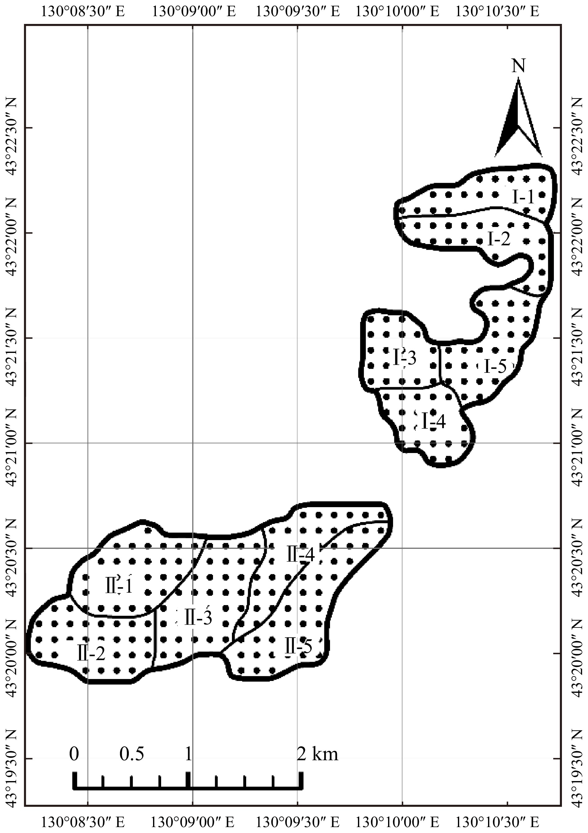
图 1 样地位置示意图
Ⅰ-1表示检查法样地第1大区第1小区,Ⅱ-1表示第2大区第1小区,以此类推。Ⅰ-1 indicates the first subregion within the first major area in the inspection area, Ⅱ-1 indicates the first subregion within the second major area in the inspection area, and so on.
Figure 1. Schematic diagram of sample site location
![]()
图 2 TWINSPAN分类过程和结果
“D”为样本分组,“N”为样本数量;“−”表示负指示种,“+”表示正指示种,即负(正)指示树种的多度达到一定程度时,将此样本分到左(右)侧。下同。“D” is a sample group, and “N” is sample size; “−” indicates a negative indicator, “+” indicates a positive indicator, meaning that when the abundance of negative (positive) indicative tree species reaching a certain level, the sample will be divided to the left (right) side. The same below.
Figure 2. Process and results of TWINSPAN classification
表 1 样地因子统计量
Table 1 Sample plot factor statistics
因子
Factor平均值
Mean最大值
Max. value最小值
Min. value平均胸径 Mean DBH/cm 18.80 33.30 9.60 公顷蓄积量/(m3·hm−2)
Hectare volume /(m3·ha−1)226.44 580.46 27.79 公顷株数/(株·hm−2)
Plant number per hectare/(tree·ha−1)682.00 2 050.00 175.00 平均树高 Average tree height/m 13.70 19.70 8.60 公顷生物量/(t·hm−2)
Hectare biomass/(t·ha−1)65.32 175.30 9.07 针叶树种占比
Proportion of coniferous tree species/%80.14 100.00 40.73 云冷杉占比
Proportion of spruce and fir/%63.49 100.00 23.20  下载: 导出CSV
表 2 吻合系数计算原理
Table 2 Principle of calculating anastomosis coefficients
样本数 Number of sample 方法2 Method 2 类1 Class 1 类2 Class 2 类3 Class 3 方法1
Method 1类1 Class 1 a b c 类2 Class 2 d e f 类3 Class 3 g h i 注:a、b、c、d、e、f、g、h、i表示对应分类的样本数。Notes: a, b, c, d, e, f, g, h, i represent the number of samples of the corresponding classification.
下载: 导出CSV
表 3 5种方法分类结果中各阶段的主要林分指标
Table 3 Main stand indicators for each stage in the classification results of 5 methods
方法
Method阶段/类
Stage/
class平均
胸径
Mean
DBH/cm公顷蓄积量/
(m3·hm−2)
Hectare volume/
(m3·ha−1)公顷株数/
(株·hm−2)
Plant number
per hectare/
(plant·ha−1)针阔比
Ratio of
coniferous to
broad-leaved tree/%平均
树高
Average
tree
height/m公顷断面积/
(m2·hm−2)
Hectare
cross-sectional
area/(m2·ha−1)公顷生物量/
(t·hm−2)
Hectare
biomass/
(t·ha−1)物种多样
性指数
Species
diversity
index径级大小
多样性
指数
Diversity
index of
diameter
size种间联结−最优分割法
Interspecies linkage-optimal
segmentation1 17.4 141.63 574 71.24 13.2 15.61 50.12 1.44 2.09 2 19.1 246.27 727 82.05 13.8 25.19 71.97 1.43 2.30 3 20.8 339.78 796 92.29 14.4 32.92 81.15 1.22 2.36 林相特征判别法
Forest phase
discrimination method1 14.5 196.78 1 053 68.61 11.9 22.48 66.49 1.54 2.30 2 18.5 221.50 651 81.72 13.6 22.65 62.77 1.37 2.24 3 24.6 276.37 452 84.60 16.1 26.10 75.09 1.28 2.09 TWINSPAN双向
指示物种分析法
TWINSPAN bidirectional
indicator species
analysis method1/类1 Class 1 17.8 172.77 611 73.31 13.4 18.45 57.28 1.48 2.14 2/类3 Class 3 19.3 273.18 789 87.37 13.8 27.60 72.22 1.31 2.35 3/类2 Class 2 22.2 329.08 659 88.67 15.0 31.09 81.13 1.20 2.20 MRT多元回归树法
MRT multiple regression
tree method1/类1 Class 1 17.8 158.75 586 75.66 13.4 17.01 50.90 1.42 2.11 2/类3 Class 3 19.6 310.31 829 85.02 14.0 31.04 84.38 1.37 2.40 3/类2 Class 2 26.6 303.05 383 94.62 16.7 26.91 65.03 1.02 1.99 基于TWINSPAN的
判别分析法
Discriminant analysis
method based on
TWINSPAN1 17.9 164.97 575 72.93 13.5 17.63 56.20 1.46 2.12 2 19.0 288.20 860 88.18 13.7 29.24 74.81 1.32 2.40 3 24.0 359.05 583 91.94 15.5 32.83 83.48 1.16 2.16
下载: 导出CSV
表 4 5种方法分类结果中各阶段的树种组成
Table 4 Composition of tree species at each stage in the classification results of five methods
方法 Method 阶段/类 Stage/class 树种组成 Tree species composition 种间联结−最优分割法
Interspecies linkage-optimal segmentation1 3云3冷1红1桦1椴1白 + 色 + 水−榆−杨 2 3冷3云2松1椴1桦−色−白 3 4冷3云2红 + 椴−桦−色 林相特征判别法
Forest phase characteristic discrimination method1 4冷2云1红1椴1桦 + 白 + 色−杂−水−榆 2 4冷3云2红1椴 + 桦 + 白 + 色 3 4云3冷2红 + 桦 + 椴−色−榆−水 TWINSPAN双向指示物种分析法
TWINSPAN bidirectional indicator species analysis1/类1 Class 1 3云3冷1红1桦1椴 + 白 + 色 + 水−榆−杨−杂 2/类3 Class 3 5冷2红2云 + 椴 + 桦−白−色 3/类2 Class 2 5云2冷2红1椴−桦−色 MRT多元回归树法
MRT multiple regression tree method1/类1 Class 1 3云3冷1红1桦1椴 + 白 + 色−水−榆 2/类3 Class 3 4云3冷2红1椴 + 桦−色−白 3/类2 Class 2 6云2红2冷 + 桦 基于TWINSPAN的判别分析法
Discriminant analysis method based on TWINSPAN1 3云3冷1红1桦1椴 + 白 + 色−水−榆 2 4冷3云2红 + 椴 + 桦−色−白 3 4云3冷2红 + 椴 + 桦 注:云.鱼鳞云杉和红皮云杉;冷.臭冷杉;红.红松;桦.硕桦;椴.椴树;白.白桦;色.色木槭;水.水曲柳;榆.榆;杨.大青杨;杂.青楷槭和花楷槭。Notes: 云, Picea jezoensis var. microsperma and Picea koraiensis; 冷, Abies nephrolepis; 红, Pinus koraiensis; 桦, Betula costata; 椴, Tilia tuan; 白, Betula platyphylla; 色, Acer mono; 水, Fraxinus mandschurica; 榆, Ulmus pumila; 杨, Populus ussuriensis. 杂, Acer tegmentosum and A. ukurunduense.
下载: 导出CSV
表 5 5种方法划分结果中各阶段间林分指标的多重比较显著性
Table 5 Significance of multiple comparisons of stand indicators between different stages in the results of five classification methods
方法
Method阶段
配对
Stage-
pairing平均胸径
Mean
DBH公顷蓄积量
Hectare
volume公顷株数
Plant number
per hectare针阔比
Ratio of
coniferous to
broad-leaved
tree平均树高
Average
tree
height公顷断面积
Hectare
cross-sectional
area公顷生物量
Hectare
biomass物种多样
性指数
Species
diversity
index径级大小
多样性指数
Diversity
index of
diameter
size种间联结−最优分割法
Interspecies
linkage-optimal
segmentation1−2 *** *** *** *** *** *** *** ns *** 1−3 *** *** *** *** *** *** *** *** *** 2−3 *** *** *** *** *** *** *** *** *** 林相特征判别法
Forest phase
characteristic
discrimination method1−2 *** *** *** *** *** ns * *** *** 1−3 *** *** *** *** *** *** *** *** *** 2−3 *** *** *** *** *** *** *** *** *** TWINSPAN双向指示
物种分析法
TWINSPAN bidirectional
indicator species
analysis method1−2 *** *** *** *** *** *** *** *** ** 1−3 *** *** * *** *** *** *** *** *** 2−3 *** *** *** ns *** *** *** *** *** MRT多元回归树法
MRT multiple
regression tree method1−2 *** *** *** *** *** *** *** *** *** 1−3 *** *** *** *** *** *** *** *** *** 2−3 *** ns *** *** *** *** *** *** *** 基于TWINSPAN的
判别分析法
Discriminant analysis
method based on
TWINSPAN1−2 *** *** *** *** ** *** *** *** *** 1−3 *** *** ns *** *** *** *** *** ns 2−3 *** *** *** *** *** *** *** *** *** 注:*表示P < 0.05;**表示P < 0.01;***表示P < 0.001;ns表示P > 0.05。Notes: * means P < 0.05; ** means P < 0.01; *** means P < 0.001; ns means P > 0.05.
下载: 导出CSV
表 6 不同方法划分结果的吻合系数
Table 6 Anastomosis coefficients for the results of different methods
项目 Item 方法A Method A 方法B Method B 方法C Method C 方法D Method D 方法E Method E 方法A Method A 1 方法B Method B 0.421 1 方法C Method C 0.605 0.402 1 方法D Method D 0.601 0.429 0.700 1 方法E Method E 0.655 0.408 0.730 0.807 1 注:方法A—方法E依次为种间联结−最优分割法、林相特征判别法、TWINSPAN双向指示物种分析法、MRT多元回归树法、基于TWINSPAN的判别分析法。Notes: methods A to E as followed are interspecies linkage-optimal segmentation, forest phase characteristic discrimination method, TWINSPAN bidirectional indicator species analysis method, MRT multiple regression tree method, MRT multiple regression tree method, and discriminant analysis method based on TWINSPAN.
下载: 导出CSV
-
[1] 沈国舫. 森林培育学[M]. 北京: 中国林业出版社, 2001. Shen G F. Silviculture[M]. Beijing: China Forestry Publishing House, 2001.
[2] 温远光, 元昌安, 李信贤, 等. 大明山中山植被恢复过程植物物种多样性的变化[J]. 植物生态学报, 1998, 22(1): 34−41. Wen Y G, Yuan C A, Li X X, et al. Changes of plant species diversity during vegetation restoration in the middle mountains of Daming Mountain[J]. Chinese Journal of Plant Ecology, 1998, 22(1): 34−41.
[3] National Research Council. People and pixels: linking remote sensing and social science[M]. Washington: National Academies Press, 1998.
[4] Saldarriaga J G, West D C, Tharp M L, et al. Long-term chronosequence of forest succession in the upper Rio Negro of Colombia and Venezuela[J]. Journal of Ecology, 1988, 76(4): 938−958.
[5] Uhl C, Buschbacher R, Serrao E A S. Abandoned pastures in eastern Amazonia (Ⅰ): patterns of plant succession[J]. The Journal of Ecology, 1988, 76(1): 663−681.
[6] Moran E F, Brondizio E S, Tucker J M, et al. Effects of soil fertility and land-use on forest succession in Amazonia[J]. Forest Ecology and Management, 2000, 139(1−3): 93−108. doi: 10.1016/S0378-1127(99)00337-0
[7] Goodell L, Faber-Langendoen D. Development of stand structural stage indices to characterize forest condition in Upstate New York[J]. Forest Ecology and Management, 2007, 249(3): 158−170. doi: 10.1016/j.foreco.2007.04.052
[8] Podlaski R. Suitability of the selected statistical distributions for fitting diameter data in distinguished development stages and phases of near-natural mixed forests in the Świętokrzyski National Park (Poland)[J]. Forest Ecology and Management, 2006, 236(2−3): 393−402. doi: 10.1016/j.foreco.2006.09.032
[9] Feldmann E, Glatthorn J, Hauck M, et al. A novel empirical approach for determining the extension of forest development stages in temperate old-growth forests[J]. European Journal of Forest Research, 2018, 137(3): 321−335. doi: 10.1007/s10342-018-1105-4
[10] Zeller L, Pretzsch H. Effect of forest structure on stand productivity in Central European forests depends on developmental stage and tree species diversity[J]. Forest Ecology and Management, 2019, 434: 193−204. doi: 10.1016/j.foreco.2018.12.024
[11] 张家来. 应用最优分割法划分森林群落演替阶段的研究[J]. 植物生态学与地植物学学报, 1993, 17(3): 34−41, 100−101. Zhang J L. Study on the application of optimal segmentation method to divide forest community succession stages[J]. Journal of Plant Ecology and Geobotany, 1993, 17(3): 34−41, 100−101.
[12] 马姜明, 刘世荣, 史作民,等. 川西亚高山暗针叶林恢复过程中不同恢复阶段的定量分析[J]. 应用生态学报, 2007, 18(8): 1695−1701. Ma J M, Liu S R, Shi Z M, et al. Quantitative analysis of different restoration stages during the restoration of alpine dark coniferous forest in western Sichuan[J]. Chinese Journal of Applied Ecology, 2007, 18(8): 1695−1701.
[13] 余树全. 浙江淳安天然次生林演替的定量研究[J]. 林业科学, 2003, 39(1): 17−22. Yu S Q. Quantitative study on succession of natural secondary forest in Chun’an, Zhejiang Province[J]. Forestry Science, 2003, 39(1): 17−22.
[14] 龚直文. 长白山退化云冷杉林演替动态及恢复研究[D]. 北京: 北京林业大学, 2009. Gong Z W. Study on succession dynamics and restoration of degraded spruce forest in Changbai Mountain[D]. Beijing: Beijing Forestry University, 2009.
[15] 唐守正. 多元统计分析方法[M]. 北京: 中国林业出版社, 1984: 238−249. Tang S Z. Multivariate statistical analysis method[M]. Beijing: China Forestry Publishing House, 1984: 238−249.
[16] Lu D, Mausel P, Brondızio E, et al. Classification of successional forest stages in the Brazilian Amazon basin[J]. Forest Ecology and Management, 2003, 181(3): 301−312. doi: 10.1016/S0378-1127(03)00003-3
[17] 李婷婷, 陆元昌, 张显强,等. 经营的马尾松森林类型发育演替阶段量化指标研究[J]. 北京林业大学学报, 2014, 36(3): 9−17. doi: 10.13332/j.cnki.jbfu.2014.03.002 Li T T, Lu Y C, Zhang X Q, et al. Quantitative indices to identify succession stages of managed Pinus massoniana forest[J]. Journal of Beijing Forestry University, 2014, 36(3): 9−17. doi: 10.13332/j.cnki.jbfu.2014.03.002
[18] 周梦丽, 雷相东, 国红,等. 基于TWINSPAN分类的天然云冷杉−阔叶混交林发育阶段划分[J]. 林业科学研究, 2019, 32(3): 49−55. doi: 10.13275/j.cnki.lykxyj.2019.03.007 Zhou M L, Lei X D, Guo H, et al. Developmental stage division of natural spruce-broadleaf mixed forest based on TWINSPAN classification[J]. Forest Research, 2019, 32(3): 49−55. doi: 10.13275/j.cnki.lykxyj.2019.03.007
[19] 张会儒, 汤孟平. 金沟岭林场混交林TWINSPAN分类及演替序列分析[J]. 南京林业大学学报(自然科学版), 2009, 33(1): 37−42. Zhang H R, Tang M P. TWINSPAN classification and succession sequence analysis of mixed forest in Jingouling Forest Farm[J]. Journal of Nanjing Forestry University (Natural Science Edition), 2009, 33(1): 37−42.
[20] 张金屯. 植被数量生态学方法[M]. 北京: 科学出版社, 1995. Zhang J T. Quantitative ecological method of vegetation[M]. Beijing: Science Press, 1995.
[21] 赖江山, 米湘成, 任海保,等. 基于多元回归树的常绿阔叶林群丛数量分类: 以古田山24公顷森林样地为例[J]. 植物生态学报, 2010, 34(7): 761−769. Lai J S, Mi X C, Ren H B, et al. Classification of evergreen broad-leaved forest cluster based on multiple regression trees: a case study of 24 hectares of forest plot in Gutianshan[J]. Chinese Journal of Plant Ecology, 2010, 34(7): 761−769.
[22] Zenner E K, Sagheb-Talebi K, Akhavan R, et al. Integration of small-scale canopy dynamics smoothes live-tree structural complexity across development stages in old-growth Oriental beech (Fagus orientalis Lipsky) forests at the multi-gap scale[J]. Forest Ecology and Management, 2015, 335: 26−36. doi: 10.1016/j.foreco.2014.09.023
[23] 颜攀. 基于近自然林经营的鲁南山地侧柏人工林经营模型构建与营林效果评价[D]. 泰安: 山东农业大学, 2020. Yan P. Construction of management model and evaluation of forestry effect of Lunan Mountain cypress plantation based on near-natural forest management[D]. Tai’an: Shandong Agricultural University, 2020.
[24] 周超凡, 冯林艳, 何潇,等. 目标树经营对云冷杉针阔混交林单木生长的影响研究[J]. 林业科学研究, 2022, 35(2): 19−27. doi: 10.13275/j.cnki.lykxyj.2022.02.003 Zhou C F, Feng L Y, He X, et al. Effects of target tree management on single growth of spruce coniferous and broad-leaved mixed forest[J]. Forest Research, 2022, 35(2): 19−27. doi: 10.13275/j.cnki.lykxyj.2022.02.003
[25] Greig-Smith P. Quantitative plant ecology[M]. Los Angeles: University of California Press, 1983.
[26] 王伯荪, 彭少麟. 南亚热带常绿阔叶林种间联结测定技术研究——Ⅰ. 种间联结测式的探讨与修正[J]. 植物生态学与地植物学丛刊, 1985(4): 274−285. Wang B S, Peng S L. Study on interspecific linkage measurement technology of tropical evergreen broad-leaved forest in South Asia (Ⅰ): discussion and correction of interspecific linkage measurement pattern[J]. Plant Ecology and Geobotany Series, 1985(4): 274−285.
[27] 潘紫重, 应天玉, 赵艳霞. 帽儿山复层异龄天然林的林龄结构[J]. 东北林业大学学报, 2008, 36(6): 9−12. Pan Z C, Ying T Y, Zhao Y X. Forest age structure of multi-layered heterogeneous natural forest in Maoershan[J]. Journal of Northeast Forestry University, 2008, 36(6): 9−12.
[28] 胡云云, 亢新刚, 赵俊卉. 长白山地区天然林林木年龄与胸径的变动关系[J]. 东北林业大学学报, 2009, 37(11): 38−42. Hu Y Y, Kang X G, Zhao J H. Relationship between age and breast diameter of natural forest in Changbai Mountain[J]. Journal of Northeast Forestry University, 2009, 37(11): 38−42.
[29] 尹艳豹, 唐守正, 郎璞梅,等. 多回波机载LiDAR数据提取林地DEM的判别分析方法[J]. 林业科学, 2011, 47(12): 106−113. Yin Y B, Tang S Z, Lang P M, et al. Discriminant analysis method of multi-echo airborne LiDAR data extraction from forest land DEM[J]. Forestry Science, 2011, 47(12): 106−113.
[30] Hill M O. A FORTRAN program for arranging multivariate data in an ordered two-way table by classification of the individuals and attributes[Z/OL]. Twinspan, 1979[2023−03−19]. https://github.com/jarioksa/twinspan/blob/master/README.md.
[31] Dufrene M, Legendre P. Species assemblages and indicator species: the need for a flexible asymmetrical approach[J]. Ecological Monographs, 1997, 67(3):345−366.
[32] Roleček J, Tichý L, Zelený D, et al. Modified TWINSPAN classification in which the hierarchy respects cluster heterogeneity[J]. Journal of Vegetation Science, 2009, 20(4): 596−602. doi: 10.1111/j.1654-1103.2009.01062.x
[33] De’ath G. Multivarlate regression trees: a new technique for modeling species–environment relationships[J]. Ecology, 2002, 83: 1105−1117.
[34] De’ath G, Fabricius K E. Classification and regression trees: a powerful yet simple technique for ecological data analysis[J]. Ecology, 2000, 81: 3178−3192. doi: 10.1890/0012-9658(2000)081[3178:CARTAP]2.0.CO;2
[35] 薛茜, 刘万里, 尔西丁, 等. 常用多重比较方法[J]. 中国医院统计, 2008(1): 29−31. Xue Q, Liu W L, Erxiding, et al. Common multiple comparison methods[J]. China Hospital Statistics, 2008(1): 29−31.
[36] 张文静, 张钦弟, 王晶,等. 多元回归树与双向指示种分析在群落分类中的应用比较[J]. 植物生态学报, 2015, 39(6): 586−592. doi: 10.17521/cjpe.2015.0056 Zhang W J, Zhang Q D, Wang J, et al. Comparison of multiple regression tree and bidirectional indicator species analysis in community classification[J]. Chinese Journal of Plant Ecology, 2015, 39(6): 586−592. doi: 10.17521/cjpe.2015.0056
[37] 张金屯. 模糊C-均值聚类和TWINSPAN分类的比较研究[J]. 武汉植物学研究, 1994(1): 11−17. Zhang J T. Comparative study of fuzzy C-means clustering and TWINSPAN classification[J]. Wuhan Botanical Research, 1994(1): 11−17.
[38] De’ath G. Multivariate regression trees: a new technique for modeling species-environment relationships[J]. Ecology, 2002, 83(4): 1105−1117.
[39] Král K, Vrška T, Hort L, et al. Developmental phases in a temperate natural spruce-fir-beech forest: determination by a supervised classification method[J]. European Journal of Forest Research, 2010, 129(3): 339−351. doi: 10.1007/s10342-009-0340-0
[40] 张金屯. 数量生态学[M]. 北京: 科学出版社, 2004. Zhang J T. Quantitative ecology[M]. Beijing: Science Press, 2004.
[41] Lu D. Estimation of forest stand parameters and application in classification and change detection of forest cover types in the Brazilian Amazon Basin[M]. Terre Haute: Indiana State University, 2001.
[42] Foody G M, Palubinskas G, Lucas R M, et al. Identifying terrestrial carbon sinks: classification of successional stages in regenerating tropical forest from Landsat TM data[J]. Remote Sensing of Environment, 1996, 55(3): 205−216. doi: 10.1016/S0034-4257(95)00196-4
-
期刊类型引用(2)
1. 黎浩然,曾志斌,季璇,李泓昊. 一个珍贵的岭南明代木结构建筑病害诊断及修缮案例剖析. 广州建筑. 2025(01): 91-96 .  百度学术
百度学术
2. 周海宾,韩旭,黄磊,王卫滨,王双永. 古建筑木构件开裂机制、评估与加固研究进展. 木材科学与技术. 2024(01): 13-22 . 百度学术
其他类型引用(1)
-
其他相关附件
-
压缩文件
基于twinspan的判别分析法 点击下载(0KB) -
压缩文件
twinspan 点击下载(0KB) -
压缩文件
种间联结-最优分割法 点击下载(1KB) -
压缩文件
林相特征判别法 点击下载(0KB) -
压缩文件
MRT多元回归树 点击下载(0KB)
-


计量
- 文章访问数: 624
- HTML全文浏览量: 143
- PDF下载量: 130
- 被引次数: 3
