
Daily variations of δ18O and its quantitative distinction in evapotranspiration components of Platycladus orientalis plantation during the rapid growth season in the mountainous area of Beijing
-
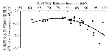
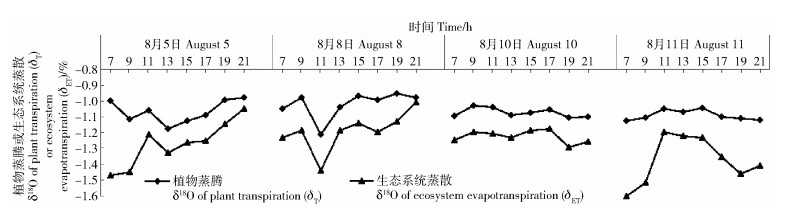
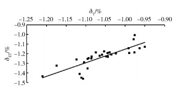
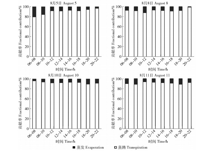
摘要: 侧柏是北京山区分布范围较广的典型针叶树种,研究侧柏林生长旺季蒸散过程及蒸散组分变化特征对了解该区陆地生态系统水汽交换、植被耗水需求具有重要意义。本研究利用稳定同位素技术于生长旺季(2016年8月)对侧柏林大气水汽δ18O进行原位连续观测,同时选取4个典型晴天采集枝条和土壤样品并测定样品水中的δ18O。结果表明:日尺度上,利用Craig-Gordon模型计算的土壤蒸发水汽氧同位素组成(δE)在4个测定日中均先增大后减小,δE>介于-5.968%~-2.689%,最大峰值出现在12:00—14:00,而近地面大气相对湿度(h)先减小后增大,二者关系为δE=-0.03h2+4.85h-209.5(R2=0.55,n=32),表明h>75%时,环境相对湿度越大,同位素分馏效应越明显;基于稳态假设估算的植物蒸腾水汽氧同位素组成(δT)和Keeling曲线拟合的侧柏林蒸散水汽氧同位素组成(δET)分别介于-1.210%~-0.951%、-1.599%~-1.004%,日变化趋势复杂,日间变化差异大,但同一观测日内δT和δET变化趋势基本一致,表明植物蒸腾非稳态可能对δT的估算产生偏离,δET变化主要受δT影响;4个测定日中蒸腾量占总蒸散量的比例(FT)介于90.14%~92.63%,说明研究区侧柏林生态系统生长旺季蒸散发绝大部分来自植物蒸腾。研究结果确定了基于日尺度的生长旺季植被蒸腾对蒸散的贡献率,为研究陆地生态系统水汽交换机制提供了有益参考,为区域森林生态建设和管理提供了科学依据。Abstract: As the dominant coniferous tree species in the mountainous area of Beijing, it is imperative to have an insight into the evapotranspiration of Platycladus orientalis in the rapid growth season and its components for deeper understanding of atmospheric vapor exchange of terrestrial ecosystems and plant water demand. The variations of daily δ18O in a Platycladus orientalis plantation during the rapid growth season and proportions of plant transpiration and soil evaporation to evapotranspiration were analyzed. The continuous water vapor stable isotope analyzer was used to measure δ18O values of the atmospheric vapor in August, 2016. Mature and suberized twigs of plant and soil samples were collected and measured simultaneously to analyze δ18O values of transpiration (δT) and soil evaporation (δE), where δT and δE were determined respectively via the steady state hypothesis of isotope and the Craig-Gordon equation. The oxygen isotopic compositions of total evapotranspiration (δET) could be estimated by a Keeling plot linear regression function.The results showed that: values of δE ranged from -5.968% to -2.689%, which rised firstly and then declined at the daily scale; and δ18O values peaked between 12:00 and 14:00, whereas the atmospheric relative humidity (h) dropped firstly and then rised. The relationship between δE and h was δME= -0.03h2+4.85h-209.5 (R2=0.55, n=32), which indicated that the isotopic fractionation was intensified with h when its value was above 75%. Although the diurnal variations of δET and δT values were complex and there was inconsistent variation tendency for the two in the four experimental days (ranged from -1.210% to -0.951% and -1.599% to -1.004%, respectively), both of them basically shared identical changing trend at the same observation days, suggesting that the evaluation of δT values was probably affected by non-steady state of stable isotopes in the leaf water. And the variations on δET were dominantly driven by δT rather than δE. The results of evapotranspiration partition showed that the contribution of plant transpiration (FT) ranged from 90.14% to 92.63% during the experimental days, indicating that the main component of evapotranspiration was plant transpiration during the rapid growth season. The results may have further implications for future forest construction and management in this area.
-
通常情况下,图像识别分类时存在着类内相似、类间差异的特点,但是在树种图像识别中,往往存在着类内差异、类间相似的现象[1]。同类树种之间,由于年龄大小、季节变化等因素,导致图像之间会有很大的差异;不同树种之间,尤其是同科树种之间,在局部特征和细节方面,却存在相似之处。这就给基于单一人工特征的传统识别方法带来了更大的难度。寻求新的方法快速准确地对树种图像进行自动识别是研究的关键所在。
现有的树种识别研究比较热门的有基于遥感影像和基于数字图像两个方面。Richter等[2]利用高光谱数据,通过引入基于偏最小二乘的判别分析,对树种进行分类,总体准确率达到78.4%;Pham等[3]将激光雷达和光谱数据相结合,利用随机森林确定重要的特征变量,支持向量机作为分类器,总体精确度为85.4%(Kappa系数为80.6%)。在基于数字图像方面,又可分为传统人工特征识别和神经网络智能识别。传统人工特征识别方面,陈明健等[4]将叶片传统特征、距离矩阵和角点矩阵相融合,对树种进行识别,识别率达到90%以上;李可心等[5]以树皮图像为研究对象,通过灰度共生矩阵,提取树皮图像的纹理信息,并利用SOM神经网络,对3类树种进行识别,识别率较为理想;杨洋[6]基于Haar小波变换的方法,并将SVM作为分类器,对树种进行识别,通过对叶片提取几何特征和纹理特征,并采用SVM的分类方法,取得了理想的识别准确率;于海鹏等[7]通过对木材图像提取色调、饱和度等9个特征参数,从纹理特征的最大相似性入手,对木材树种进行分类识别,检索正确率较高;孙伶君等[8]对木材图像采用分块LBP特征提取,使用衰减、卡方、欧式3种方法分类,最近邻法识别,准确率高达93.3%。神经网络智能识别方面,在国外,Bertrand等[9]将树干、树叶特征相结合,并将算法嵌入到智能手机中,大大增强了实用化和利用率。Zhao等[10]将树种叶片作为研究对象,基于Android系统,开发一款名为“Apleap”的移动端软件,不仅为专业人士识别带来便利,对普通民众来说,普及率大大提高;在国内,对于树种智能识别的研究起步相对较晚,赵鹏超等[11]以阔叶叶脉的纹理特征为切入点,构建卷积神经网络,最终训练识别率达到95%以上,为树种识别提供新思路。上述方法,尽管都取得了不错的识别效果,但也存在着一些问题,如大部分研究是依靠人工提取图像特征来满足实验要求。众所周知,同一棵树,在不同季节、不同年龄、不同拍摄角度等条件下,都会显示出不同的形态,其图像中各个特征信息都会随之发生变化,因此对继续提高树种识别率带来了困难。
近年来,深度卷积神经网络发展迅速,得到了广泛关注。物体不管呈现出何种状态,深度学习方法获取的低层和深层的特征信息都能够做到保持不变[12]。早期,Lecun等[13]提出L提出LeNet-5模型,基于反向传播算法对网络进行训练,通过卷积层和池化层将原始图像特征进行自动提取,并转化为相对应的特征子图,最后将全连接层作为“分类器”,进行最后的分类输出,并最终在MNIST手写字符数据集的识别上取得了成功。2012年,卷积神经网络迎来了发展高潮,Krizhevsky等[14]首次将深度学习理念应用到图像分类中,提出AlexNet模型,并在ImageNet[15]图像分类大赛中,以巨大优势获得冠军,使得卷积神经网络在图像处理领域成为最受欢迎的方法。在接下来的几年里,在经典卷积神经网络模型的基础上,不断有学者和研究人员进行改进和创新,如Simonyan等[16]提出的VGG模型、Szegedy等[17]提出的GoogLeNet模型、He等[18]提出的ResNet模型等。鉴于卷积神经网络在图像识别分类上的广泛应用,陆续有研究人员在树种图像识别中采用CNN。例如,上面提到的赵鹏超等人,将叶脉的纹理特征作为CNN的输入值,其分类效果明显高于传统人工特征方法,一定程度上表明深度学习方法的可行性。但是,此研究采用单一特征进行识别,不够全面,是否能应用到其他特征识别上来,还有待进一步验证。
基于上述问题,本文基于CNN模型,提出一种将图像深层特征和人工特征融合的树种图像深度学习识别方法,使用3路相同的CNN模型作为并行网络,对RGB图像、HSV图像、人工特征Gabor特征和颜色矩分别进行特征提取,并在最后一个全连接层进行汇总,识别输出。通过多特征融合解决了树种单一特征识别的限制问题,完成了对不同树种图像的自动识别。
1. 材料与方法
1.1 图像数据集
6类树种包括:樟子松(Pinus sylvestris var. mongolica)、山杨(Populus davidiana)、白桦(Betula platyphylla)、落叶松(Larix gmelinii)、雪松(Cedrus deodara)和白皮松(Pinus bungeana)。示例图像见图1A ~ F。为满足深度学习模型训练要求,通过裁剪、水平翻转、旋转对原始图像进行扩增。树种图像数据集共计3 375幅,其中训练集2 775幅,测试集600幅,各个树种图像具体数量见图2。最后,利用python脚本语言将图像像素值调整至256 × 256像素,JPG格式保存。所有图像均采集于自然状态下,拍摄设备为数码相机和智能手机。
1.2 卷积神经网络
典型的卷积神经网络(CNN)主要由输入层、卷积层、池化层(降采样层)、全连接层和输出层组成[19]。
通常情况下,CNN网络的输入层为图像,紧接着是卷积层,卷积层通过对卷积核设置不同的个数和大小,将输入的图像转化为特征子图(feature map),传递到下一层。卷积的计算公式可以表示为:
Ilj=∑iIl−1i⊗kl−1ij+blj (1) 式中:
Ilj 代表第l层产生的第j个特征图;kl−1ij 代表卷积核个数;blj 为偏置项;⊗ 代表卷积运算。池化层通常紧连接着卷积层,选择某种池化方法[20],对卷积得到的特征图进行池化,此操作也被称为下采样。池化的主要目的就是降低特征图的维度和在一定程度上保持特征的尺度不变性。池化层计算公式一般为:
Zlj=down(Ylj) (2) 式中:
Zlj 为池化层的输出项;Ylj 为池化层的输入项;down(Δ) 为池化函数。经过卷积和池化操作后,卷积神经网络会采用全连接层,作为“分类器”,对前面提取的大量特征进行分类,来确定最终的图像类别。计算公式如下:
h(IL)=f(WTIL+b) (3) 式中:
h(Δ) 为全连接层的输出项;IL 为第L层的卷积输出;W和b分别为全连接层的权重和偏置项;f(Δ) 为激励函数。除上述常规网络层之外,为提高CNN网络模型的性能和泛化能力,往往采用辅助方法。本文在每个卷积层采用ReLU激励函数,此函数不会随着输入项的增加而接近饱和[21]。ReLU激励函数计算公式如下:
f(x)=max (4) 式中:x为输入值。
另外,在ReLU函数后,也采用LRN(Local Response Normalization)[22]策略方法,旨在增强网络模型的泛化能力,计算公式如下:
b_{x,y}^i = \frac{{a_{x,y}^i}}{{{{\left( {k + \alpha \displaystyle\sum\limits_{j = \max \left( {0,i - n/2} \right)}^{\min \left( {N - 1,i + n/2} \right)} {{{\left( {a_{x,y}^j} \right)}^2}} } \right)}^\beta }}} (5) 式中:b代表特征图中i泛化后对应的像素值;j代表j ~ i的像素值的平方和;x,y为像素的位置;a代表特征图中i对应的像素值;N为特征图里面最内层向量的列数;k,α,n,β均为超参数,本文取值分别为:k = 2,α = 0.000 1,n = 5,β = 0.75。
1.3 特征提取
1.3.1 RGB图像
RGB图像,即代表红(R)、绿(G)、蓝(B)3个通道的颜色,通过不同颜色分量来表示彩色图像。本文原始数据集,即RGB图像,直接作为本文第1路CNN网络的输入图像。
1.3.2 HSV图像
HSV图像,即代表色调(H)、饱和度(S)、亮度(V),较RGB图像相比,HSV图像更加符合人类对于颜色的直观感受。之所以选择HSV图像作为另一种特征,是因为在拍摄树种图像时,亮度的变化对树种识别产生一定程度的影响。因此,本文将树种图像从RGB颜色空间转化为HSV颜色空间,作为本文第2路CNN网络的输入图像。转换思路如下:
\begin{split} & H = \left\{ \begin{array}{*{20}{l}} \!\!\!\!\!{0^ \circ ,} & \!\!\!\!\!{{\rm{if}}\;{\rm{MAX}} = {\rm{MIN}}}\\ \!\!\!\!{{60^ \circ } \times \dfrac{{G - B}}{{{\rm{MAX}} - {\rm{MIN}}}} + {0^ \circ },} &\!\!\!\!\! {{\rm{if}}\;{\rm{MAX}} = R\;{\rm{and}}\;G \geqslant B}\\ \!\!\!\!{{60^ \circ } \times \dfrac{{G - B}}{{{\rm{MAX}} - {\rm{MIN}}}} + {360^ \circ },} & \!\!\!\!\!{{\rm{if}}\;{\rm{MAX}} = R\;{\rm{and}}\;G < B}\\ \!\!\!\!{{60^ \circ } \times \dfrac{{B - R}}{{{\rm{MAX}} - {\rm{MIN}}}} + {120^ \circ },} & \!\!\!\!\!{{\rm{if}}\;{\rm{MAX}} = G}\\ \!\!\!\!{{60^ \circ } \times \dfrac{{R - G}}{{{\rm{MAX}} - {\rm{MIN}}}} + {240^ \circ },} & \!\!\!\!\!{{\rm{if}}\;{\rm{MAX}} = B} \end{array} \right.\\ & S = \left\{ \begin{array}{*{20}{l}} \!\!\!\!\!{0^ \circ ,} & \!\!\!{{\rm{if}}\;{\rm{MAX}} = 0}\\ \!\!\!\!{\dfrac{{{\rm{MAX}} - {\rm{MIN}}}}{{{\rm{MAX}}}} = 1 - \dfrac{{{\rm{MIN}}}}{{{\rm{MAX}}}},} & \!\!\!\!\!{{\rm{Otherwise}}} \end{array} \right.\\ & V = {\rm{MAX}} \end{split} (6) 式中:R、G、B为红(R)、绿(G)、蓝(B)的颜色值;H、S、V为色调(H)、饱和度(S)、亮度(V)的值;MAX为R、G、B中的最大值,MIN为最小值;H在[0,360°]之间,S在[0,100°]之间,V在[0,MAX]之间。
1.3.3 LBP特征
本文采用LBP[23]来描述树种图像局部纹理特征,利用其灰度不变性、旋转不变性以及对光照变化的鲁棒性,能够表示90%以上的纹理信息。LBP计算公式如下:
{\rm{LBP}}\left( {{x_{\rm{c}}},{y_{\rm{c}}}} \right) = \sum\limits_{p = 0}^{p - 1} {{2^p}s\left( {{i_p} - {i_{\rm{c}}}} \right)} (7) s\left( x \right) = \left\{ \begin{gathered} 1\begin{array}{*{20}{c}} {}&{x \geqslant 0} \end{array} \\ 0\begin{array}{*{20}{c}} {}&{x < 0} \end{array} \\ \end{gathered} \right. (8) 式中:(xc,yc)是邻域窗口的中心元素,像素值大小为ic;ip是3 × 3邻域窗口内其他像素值;s(x)是符号函数。
LBP特征提取步骤:
(1) 首先,根据原始图像的像素大小为256 × 256,因此将检测窗口划分为16 × 16的子区域。
(2) 利用上述公式对每个子区域的像素点的LBP进行计算。
(3) 计算每个子区域的直方图,也就是每个LBP值出现的频率,并对直方图进行归一化处理。
(4) 最后将得到的所有直方图连接成为一个特征向量,即整个图像的LBP纹理信息。
1.3.4 HOG特征
本文采用HOG特征[24]来描述树种图像的形状特征,提高模型对光照因素的鲁棒性,其通过计算图像局部的方向梯度直方图来表达形状特征。HOG特征计算公式如下:
\begin{gathered} {G_{\rm{x}}}\left( {x,y} \right) = H\left( {x + 1,y} \right) - H\left( {x - 1,y} \right) \\ {G_{\rm{y}}}\left( {x,y} \right) = H\left( {x,y + 1} \right) - H\left( {x,y - 1} \right) \\ \end{gathered} (9) 式中:Gx(x,y)代表图像中像素点(x,y)水平方向梯度,Gy(x,y)代表图像中像素点(x,y)垂直方向梯度,H(x,y) 代表图像的像素值。
\begin{gathered} {G_{\rm{x}}}\left( {x,y} \right) = \sqrt {{G_{\rm{x}}}{{\left( {x,y} \right)}^2}{\rm{ + }}{G_{\rm{y}}}{{\left( {x,y} \right)}^2}} \\ \alpha \left( {x,y} \right) = {\tan ^{ - 1}}\left( {\frac{{{G_{\rm{y}}}\left( {x,y} \right)}}{{{G_{\rm{x}}}\left( {x,y} \right)}}} \right) \\ \end{gathered} (10) 式中:α(x,y)代表像素点(x,y)处的方向。
HOG特征提取步骤:
(1) 灰度化:由于颜色信息起的作用不大,因此将图像转化为灰度图像。
(2) 为减少光照等因素的影响,对整个图像进行归一化处理。
(3) 本文采用的梯度算子为:水平方向算子为[− 1, 0, 1],垂直方向算子为[− 1, 0, 1]T。再通过公式(9)和公式(10)计算梯度幅值和梯度方向。
(4) 将整个图像分割成小的Cell单元格(8 × 8像素)。
(5) 本文采用9个组距的直方图来统计8 × 8个像素的梯度信息,对单元格内的每个像素进行加权投影,得到该单元格对应的9维特征向量。
(6) 最后将得到的所有单元格组成大的块,块内归一化直方图,即整个图像的HOG纹理信息。
1.4 构建树种识别CNN模型
本文在经典卷积神经网络的基础上,进行改进和完善,根据数据集的实际情况,经过不断调试,构建了适合本文树种图像识别的3路并列网络模型(图3)。每路CNN树种识别模型,由4个卷积层、4个池化层、3个全连接层组成,具体的参数设置如下。
第1个卷积层:有64个卷积核,大小为11 × 11;步长为2,激励函数为ReLU;采用最大池化法,池化窗口大小为2 × 2;并加入LRN层。
第2个卷积层:有128个卷积核,大小为5 × 5;步长为2,激励函数为ReLU;采用最大池化法,池化窗口大小为2 × 2;特征图的高度宽度均填充2像素。
第3个卷积层:有128个卷积核,大小为5 × 5;步长为1;采用最大池化法,池化窗口大小为4 × 4;特征图的高度宽度均填充1像素,激励函数为ReLU。
第4个卷积层:有128个卷积核,大小为3 × 3;步长为2;采用最大池化法,池化窗口大小为2 × 2;特征图的高度宽度均填充1像素,激励函数为ReLU。
全连接层:前两个全连接层包含4 096个神经元,最后一个全连接层包含1 000个神经元。输出类别:6类树种名称。
1.5 识别结果评价标准
本文用验证识别准确率和平均验证识别准确率作为识别结果的评价标准。
\begin{array}{l} {\text{验证识别准确率}} = \dfrac{{\text{正确识别出树种类别的数量}}}{{\text{树种图形的总数量}}}\\ \!\!\!\!{\text{平均验证识别准确率}}\! =\! \dfrac{{\text{每类树种验证识别准确率之和}}}{{\text{树种类别总数}}} \end{array} 2. 结果与分析
本文实验是采用的编程语言是Python3.5,在TensorFlow框架下实现的。计算机操作系统为Windows 8.1,处理器为Intel(R) Core(TM) i5-3330 CPU,安装内存6 GB。CNN模型训练参数设置为:学习率0.000 1,迭代次数为6 000,Batch_size为64。整个并列网络训练时的准确率和损失率如图4所示。从图4中可以看出,在训练到5 000次时,训练准确率趋于稳定,且无较大变化。在训练开始的500次时,损失率迅速下降,经过5 000次后,损失率下降到0.1左右,并趋于一个平稳的状态。
基于本文方法的实验结果如表1所示。从最终识别结果可以看出,利用3路并列网络,将多个特征进行融合,平均验证识别准确率为91.17%,基本满足对树种图像的识别要求。其中,白皮松树种图像验证识别准确率最高,达到93.50%,落叶松识别准确率较低,达到88.70%。
表 1 本文方法的实验结果Table 1. Experimental results in this paper% 项目 Item 樟子松
Pinus sylvestris
var. mongolica山杨
Populus
davidiana白桦
Betula
platyphylla落叶松
Larix
gmelinii雪松
Cedrus
deodara白皮松
Pinus
bungeana验证识别准确率
Accuracy rate of verification and recognition91.50 90.40 92.80 88.70 90.10 93.50 平均验证识别准确率
Average accuracy rate of verification and recognition91.17 2.1 模型训练特征图显示
本文以一张白桦图像为例,分别展示了RGB图像、HSV图像、LBP图像和HOG图像在卷积层、池化层的特征图(图5 ~ 8)。由于篇幅有限,本文每层只展示4幅特征图。从图中可以得出4张图像可视化的共同点:在浅层的卷积和池化过程中,模型对图像的边缘信息最感兴趣;在越高层的卷积和池化过程中,提取的图像特征信息越来越抽象,越来越复杂,肉眼已经很难去识别。通过调用CNN的可视化功能,能够及时了解CNN识别图像的过程,也为我们改进网络模型结构提供了参考依据。
2.2 卷积核数目对实验的影响
本文对CNN模型的卷积层中卷积核数目进行不同的组合和测试,对比实验的具体参数和结果如表2所示。经过几种不同的卷积核数目的组合,64-128-128-128组合的训练准确率最高,达到了96.13%。一般情况下,卷积核数目越多,可提取学习的特征信息就越多,但也造成了网络模型中的参数骤增,计算速度变慢,容易在训练过程中造成过拟合。
表 2 不同卷积核数目的训练准确率Table 2. Training accuracy rate of different convolution kernel numbers卷积核数目
Convolution kernel number训练准确率
Training accuracy rate/%32-64-64-128 75.26 32-64-128-64 72.21 32-64-128-192 78.28 48-64-128-128 75.12 48-128-192-128 81.79 48-128-128-192 82.23 64-128-128-128 96.13 64-128-192-192 91.27 64-64-128-192 92.02 2.3 不同特征组合对实验的影响
由表3可以看出,在单一特征条件下,训练准确率和验证准确率最高的是RGB特征,分别为75.21%和72.17%;其次是HSV特征;HOG纹理特征和LBP形状特征的识别率最差。将HSV图像进行单通道提取,分别作为单一特征进行测试,虽然相对LBP-HOG特征来说,训练准确率和验证准确率有所提高,但是实验结果仍然不理想。将RGB像素值特征与其他特征进行融合,与单一特征或其他特征融合得到的模型相比,其中,“RGB + LBP形状 + H通道”的特征融合得到的识别效果最好,训练准确率和验证识别准确率分别为96.13%、93.50%。
表 3 不同特征组合的识别率Table 3. Recognition rate of different feature combinations特征
Feature训练准确率
Training accuracy rate/%验证准确集
Verification accuracy set验证集
Validation set验证识别准确率
Verifying the recognition accuracy rate/%RGB 75.21 433 600 72.17 HSV 71.56 416 600 69.33 HOG-LBP 56.28 314 600 52.33 H 63.78 377 600 62.83 S 68.12 391 600 65.17 V 64.14 375 600 62.50 RGB + H 78.26 451 600 75.17 RGB + S 75.26 440 600 73.33 RGB + V 78.21 445 600 74.17 RGB + LBP 75.23 446 600 74.33 RGB + HOG 77.58 460 600 76.67 RGB + HOG + H 86.29 498 600 83.00 RGB + HOG + S 82.15 475 600 79.17 RGB + HOG + V 84.26 493 600 82.17 RGB + LBP + H 96.13 561 600 93.50 RGB + LBP + S 88.14 525 600 87.50 RGB + LBP + V 92.36 541 600 90.17 RGB + HSV + LBP-HOG 990.56 537 600 89.50 图9给出了本文树种识别模型对6类树种测试结果的混淆矩阵[25]。混淆矩阵的每一列代表树种实际的类别,每一行代表模型预测后的类别,直观地对本文模型的识别效果进行展示。本文识别模型得到的混淆矩阵,在对角线上显示高值,在矩阵的其余部分显示低值。混淆矩阵用从蓝色到红色的颜色标度表示,蓝色表示低值,红色表示高值。从图9中可以看出,对角线上红色最多,说明识别准确率最高,也进一步说明,本文提出的树种识别算法模型取得了理想的识别效果。
![]() 图 9 树种识别结果的混淆矩阵bh:白桦Betula platyphylla;zzs:樟子松Pinus sylvestris var. Mongolica;lys:落叶松Larix gmelinii;sy:山杨Populus davidiana;bps:白皮松Pinus bungeana;xs:雪松Cedrus deodaraFigure 9. Confusion matrix of tree species recognition results
图 9 树种识别结果的混淆矩阵bh:白桦Betula platyphylla;zzs:樟子松Pinus sylvestris var. Mongolica;lys:落叶松Larix gmelinii;sy:山杨Populus davidiana;bps:白皮松Pinus bungeana;xs:雪松Cedrus deodaraFigure 9. Confusion matrix of tree species recognition results2.4 不同方法的实验结果
为验证本文提出的3路并列CNN网络模型的有效性,与SVM分类器、BP神经网络以及现有的深度学习LeNet-5模型、VGG-16模型作比较,比较结果见表4。由表4中数据可以看出,本文方法对6类树种的识别率最高。原因为:SVM和BP分类器,过度依赖于手动提取图像特征,尤其是在提取特征的过程中,不可避免的会发生一些图像关键特征的遗漏和受无关因素干扰的现象,造成识别率低;另外,LeNet-5模型,虽然是深度学习方法,但最初的设计仅仅应用于手写数字的识别,且一般情况下为灰度图像,在处理复杂的树种图像时,识别能力受到了大大的限制;VGG-16模型,是由13层卷积层和3层全连接层构成的深度学习模型,更适合于大样本量的数据识别,对于本文树种图像的小样本来说,对模型泛化能力的提高是一件困难的事,因此也没有取得理想的识别效果。本文的3路并列网络模型,从数据集中自动提取图像特征,从不同角度对图像特征进行深入挖掘并学习,使得模型泛化能力变强,识别效果理想。
表 4 与其他方法的识别率比较结果Table 4. Comparison results of recognition rates with other methods% 方法
Method识别率 Recognition rate 白桦
Betula platyphylla樟子松
Pinus sylvestris var. mongolica落叶松
Larix gmelinii雪松
Cedrus deodara山杨
Populus davidiana白皮松
Pinus bungeanaSVM 47.25 48.41 48.02 44.95 43.66 45.28 BP 36.25 39.41 40.25 39.65 39.12 38.25 LeNet-5 59.28 55.36 57.25 54.78 55.45 52.36 VGG-16 63.21 60.17 66.28 64.58 64.11 60.29 本文方法
Method in this study92.80 91.50 88.70 90.10 90.40 93.50 3. 结论与讨论
3.1 结 论
本文根据在树种图像识别时存在类内差异、类间相似的现象,提出3路并列CNN网络模型对6类树种图像进行识别。通过设计11层(4层卷积层、4层池化层、3层全连接层)CNN网络模型,分成3路,通过将RGB图像像素值特征、HSV图像色彩特征、LBP纹理和HOG形状特征进行融合,作为CNN模型的识别输入特征,在最后一层全连接层进行特征汇总,对树种种类进行识别分类。本文方法在一定程度上避免了单一特征或传统手动提取特征造成识别率低的问题,并在与SVM、BP、LeNet-5模型、VGG-16模型的比较实验中,识别效果更好,模型泛化能力得到大大提高。
众所周知,树种图像特征选择的好坏,直接影响着最终的识别结果。本文从全局特征中选择了LBP特征和HOG特征,分别从树种图像纹理和形状的角度出发,对树种图像特征做进一步表达。
本文实验研究结果表明,多特征融合的树种种类识别相对于单一特征和传统手动特征的识别方法,具有更好的识别能力。另外,多特征融合的分类器取得了对6类树种图像的最高识别率。
3.2 讨 论
尽管本文研究取得了理想的识别结果,但不同树种图像对应不同的特征,本文的CNN网络模型和参数是否仍能取得同样的识别结果,有待进一步验证。在后续的研究工作中,进一步扩大树种样本的种类和数量,继续探索更具代表性的图像特征,不断调试模型参数和权重,寻找最优的网络模型,训练出更好的CNN树种识别模型。
-
![]()
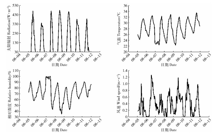
图 1 测定期间微气象数据变化
Figure 1. Variations of data on meteorological elements during measurement period
![]()
图 2 近地面大气相对湿度与土壤蒸发水汽关系曲线
Figure 2. Relationship between relative humidity and δ18O of soil evaporation
![]()
图 3 植物蒸腾和生态系统蒸散日变化
Figure 3. Daily variations of plant transpiration and ecosystem evapotranspiration
![]()
图 4 生态系统蒸散与植物蒸腾关系曲线
Figure 4. Relationship between ecosystem evapotranspiration and plant transpiration
![]()
图 5 观测期侧柏林生态系统蒸腾占蒸散的比例
Figure 5. Contributions of transpiration to evapotranspiration in the Platycladus orientalis plantation during measurement period
表 1 Craig-Gordon模型参数及δE
Table 1 Parameters of Craig-Gordon model and estimated values of soil evaporation δE
日期Date 时间Time T/K h/% δS/% δV/% δE/% 06:00—08:00 297.64±0.32 93.43±2.55 -0.647±0.030 -1.548±0.054 -3.255±0.32 08:00—10:00 298.24±0.54 83.59±3.23 -0.59±0.020 -1.465±0.072 -3.221±0.25 10:00—12:00 298.95±0.52 78.68±4.65 -0.540±0.032 -1.489±0.044 -2.835±0.32 8月5日August 5 12:00—14:00 299.33±0.67 77.48±1.76 -0.569±0.029 -1.521±0.054 -2.846±0.29 14:00—16:00 299.50±0.44 81.61±2.12 -0.506±0.058 -1.394±0.032 -3.008±0.58 16:00—18:00 299.37±0.35 81.38±2.09 -0.642±0.021 -1.550±0.067 -3.056±0.21 18:00—20:00 298.97±0.55 81.82±0.43 -0.691±0.062 -1.511±0.034 -3.507±0.62 20:00—22:00 298.53±0.51 87.58±3.64 -0.670±0.051 -1.569±0.029 -3.170±0.051 06:00—08:00 296.29±0.72 98.73±4.77 -0.651±0.032 -1.569±0.043 -3.437±0.32 08:00—10:00 296.99±0.96 86.61±3.74 -0.631±0.021 -1.492±0.055 -3.456±0.21 10:00—12:00 297.84±0.53 69.48±8.46 -0.613±0.022 -1.527±0.034 -3.077±0.22 8月8日August 8 12:00—14:00 298.66±0.32 61.08±1.59 -0.617±0.029 -1.537±0.063 -3.058±0.29 14:00—16:00 298.48±0.69 66.99±1.04 -0.621±0.018 -1.447±0.045 -3.246±0.18 16:00—18:00 297.97±0.10 66.66±4.08 -0.706±0.021 -1.572±0.059 -3.258±0.21 18:00—20:00 297.67±0.41 68.26±1.22 -0.721±0.022 -1.603±0.076 -3.251±0.22 20:00—22:00 297.36±0.32 69.31±0.97 -0.793±0.031 -1.737±0.044 -3.195±0.31 06:00—08:00 296.93±0.60 98.64±3.06 -0.603±0.027 -1.496±0.034 -4.790±0.37 08:00—10:00 297.53±0.79 86.72±3.89 -0.698±0.018 -1.522±0.066 -3.729±0.48 10:00—12:00 298.26±0.45 80.92±1.45 -0.648±0.012 -1.554±0.054 -3.115±0.32 8月10日August 10 12:00—14:00 298.89±0.34 81.94±2.45 -0.648±0.032 -1.573±0.079 -3.003±0.32 14:00—16:00 299.21±0.30 83.73±1.59 -0.646±0.019 -1.628±0.062 -2.689±0.19 16:00—18:00 299.23±0.16 83.81±1.24 -0.654±0.023 -1.622±0.097 -2.759±0.23 18:00—20:00 299.10±0.14 83.54±0.71 -0.671±0.025 -1.625±0.037 -2.860±0.25 20:00—22:00 298.88±0.23 86.47±1.69 -0.693±0.018 -1.629±0.046 -2.932±0.18 06:00—08:00 298.21±0.37 96.79±1.57 -0.632±0.019 -1.442±0.053 -5.968±0.19 08:00—10:00 298.53±0.61 93.93±3.16 -0.616±0.013 -1.416±0.032 -4.669±0.13 10:00—12:00 299.13±0.48 87.74±2.06 -0.600±0.024 -1.454±0.034 -3.386±0.24 8月11日August 11 12:00—14:00 299.84±0.20 81.83±1.43 -0.596±0.021 -1.457±0.067 -3.200±0.21 14:00—16:00 300.17±0.70 88.49±4.08 -0.585±0.031 -1.436±0.071 -3.347±0.31 16:00—18:00 300.06±0.17 91.12±1.46 -0.674±0.025 -1.493±0.038 -3.855±0.25 18:00—20:00 299.97±0.28 90.64±0.40 -0.682±0.026 -1.457±0.056 -4.246±0.26 20:00—22:00 299.73±0.41 93.80±0.34 -0.715±0.017 -1.488±0.049 -4.964±0.37 注:T、δS、δV、δE分别为土壤0.05 m深处卡尔文温度、土壤表面液态水氧同位素组成、地面以上0.05 m处大气水汽氧同位素组成、土壤蒸发水汽氧同位素组成。Notes: T, δS, δV, δE are soil Calvin temperature 0.05 m below the ground, δ18O in liquid water of soil surface, δ18O in vapor water 0.05 m above the ground, δ18O in vapor water of soil evaporation, respectively.  下载: 导出CSV
表 2 基于Keeling plots方法拟合的曲线回归分析
Table 2 Regression analysis based on Keeling Plots simulation
日期
Date时间
TimeKeeling plot方程
Keeling plot equationR2 n P 置信区间Confidence interval (95%) 置信下限Lower
confidence limit置信上限Upper
confidence limit06:00—08:00 y=-0.442 1x-14.68 0.64 360 <0.01 -15.41 -13.91 08:00—10:00 y=-0.415 1x-14.47 0.75 360 <0.01 -15.05 -13.73 10:00—12:00 y=-0.303 9x-12.09 0.79 360 <0.01 -12.71 -11.44 8月5日 12:00—14:00 y=-0.418x-13.25 0.84 360 <0.01 -13.91 -12.54 August 5 14:00—16:00 y=-0.397x-12.61 0.82 360 <0.01 -13.25 -11.93 16:00—18:00 y=-0.273x-12.47 0.80 360 <0.01 -13.09 -11.83 18:00—20:00 y=-0.273x-11.43 0.71 360 <0.01 -11.88 -10.86 20:00—22:00 y=-0.209 7x-10.47 0.65 360 <0.01 -11.03 -9.93 06:00—08:00 y=-0.246 3x-12.27 0.81 360 <0.01 -12.91 -11.66 08:00—10:00 y=-0.215x-11.83 0.61 360 <0.01 -12.38 -11.21 10:00—12:00 y=-0.119 5x-14.35 0.64 360 <0.01 -15.08 -13.62 8月8日 12:00—14:00 y=-0.226 7x-11.83 0.83 360 <0.01 -12.42 -11.21 August 8 14:00—16:00 y=-0.109 6x-11.40 0.86 360 <0.01 -11.97 -10.80 16:00—18:00 y=0.218 1x-11.91 0.81 360 <0.01 -12.44 -11.29 18:00—20:00 y=-0.277 45x-11.28 0.77 360 <0.01 -11.82 -10.70 20:00—22:00 y=-0.341 6x-11.04 0.76 360 <0.01 -10.54 -9.51 06:00—08:00 y=-0.455x-12.44 0.73 360 <0.01 -13.10 -11.79 08:00—10:00 y=-0.400 5x-11.95 0.69 360 <0.01 -12.54 -11.28 10:00—12:00 y=-0.217 1x-12.05 0.81 360 <0.01 -12.53 -11.46 8月10日 12:00—14:00 y=-0.399 1x-12.28 0.83 360 <0.01 -12.90 -11.64 August 10 14:00—16:00 y=-0.515 3x-11.85 0.8 360 <0.01 -12.44 -11.23 16:00—18:00 y=-0.344 4x-11.47 0.78 360 <0.01 -12.20 -11.15 18:00—20:00 y=-0.619 9x-12.87 0.76 360 <0.01 -13.52 -12.25 20:00—22:00 y=-0.318 6x-12.53 0.72 360 <0.01 -13.18 -11.93 06:00—08:00 y=-0.317 8x-16.00 0.76 360 <0.01 -16.79 -15.16 08:00—10:00 y=-0.194 5x-15.14 0.81 360 <0.01 -15.89 -14.36 10:00—12:00 y=-0.337 8x-11.93 0.86 360 <0.01 -12.53 -11.29 8月11日 12:00—14:00 y=-0.209 2x-12.20 0.85 360 <0.01 -12.81 -11.58 August 11 14:00—16:00 y=-0.193 8x-12.30 0.84 360 <0.01 -12.97 -11.66 16:00—18:00 y=-0.177 8x-13.53 0.8 360 <0.01 -14.20 -12.84 18:00—20:00 y=-0.176 9x-14.58 0.8 360 <0.01 -15.33 -13.83 20:00—22:00 y=-0.193 7x-14.09 0.72 360 <0.01 -14.79 -13.35
下载: 导出CSV
-
[1] 石磊, 盛后财, 满秀玲, 等.不同尺度林木蒸腾耗水测算方法述评[J].南京林业大学学报(自然科学版), 2016, 40(4): 149-156. http://d.old.wanfangdata.com.cn/Periodical/njlydxxb201604024 SHI L, SHENG H C, MAN X L, et al. A review of the calculation method of water consumption by tree transpiration in different scales[J]. Journal of Nanjing Forestry University (Natural Sciences Edition), 2016, 40(4):149-156. http://d.old.wanfangdata.com.cn/Periodical/njlydxxb201604024
[2] 王帆, 江洪, 牛晓栋.大气水汽稳定同位素组成在生态系统水循环中的应用[J].浙江农林大学学报, 2016, 33(1): 156-165. http://d.old.wanfangdata.com.cn/Periodical/zjlxyxb201601021 WANG F, JIANG H, NIU X D. Research advances in water vapor isotopic composition and its application in the hydrological research[J]. Journal of Zhejiang A &F University, 2016, 33(1): 156-165. http://d.old.wanfangdata.com.cn/Periodical/zjlxyxb201601021
[3] 巩国丽, 陈辉, 段德玉.利用稳定氢氧同位素区分白刺水分来源比较[J].生态学报, 2011, 31(24): 7533-7541. http://www.wanfangdata.com.cn/details/detail.do?_type=perio&id=stxb201124024 GONG G L, CHEN H, DUAN D Y. Comparison of the methods using stable hydrogen and oxygen isotope to distinguish the water source of Nitraria tangutorum[J]. Acta Ecologica Sinica, 2011, 31(24): 7533-7541. http://www.wanfangdata.com.cn/details/detail.do?_type=perio&id=stxb201124024
[4] 石俊杰.利用同位素原位监测技术分割农田蒸散研究[D].杨凌: 西北农林科技大学, 2012. SHI J J. Research of using isotope in situ monitoring technology partitioning field evapotranspiration[D]. Yangling: Northwest A & F University, 2012.
[5] 石俊杰, 龚道枝, 梅旭荣, 等.稳定同位素法和涡度-微型蒸渗仪区分玉米田蒸散组分的比较[J].农业工程学报, 2012, 28(20): 114-120. http://d.old.wanfangdata.com.cn/Periodical/nygcxb201220018 SHI J J, GONG D Z, MEI X R, et al. Comparison of partitioning evapotranspiration composition in maize field using stable isotope and eddy covariance-microlysimeter methods[J]. Transactions of the Chinese Society of Agricultural Engineering, 2012, 28(20): 114-120. http://d.old.wanfangdata.com.cn/Periodical/nygcxb201220018
[6] XU Z, YANG H B, LIU F D, et al. Partitioning evapotranspiration flux components in a subalpine shrubland based on stable isotopic measurements[J]. Botanical Studies, 2008, 49(4): 351-361. http://www.wanfangdata.com.cn/details/detail.do?_type=perio&id=be091f993cc66b376b47a2c9908da87e
[7] WANG P, YAMANAKA T, LI X Y, et al. Partitioning evapotranspiration in a temperate grassland ecosystem: numerical modeling with isotopic tracers[J]. Agricultural and Forest Meteorology, 2015, 208: 16-31. doi: 10.1016/j.agrformet.2015.04.006
[8] GOOD S P, SODERBERG K, GUAN K Y, et al. δ2H isotopic flux partitioning of evapotranspiration over a grass field following a water pulse and subsequent dry down[J]. Water Resources Research, 2014, 50(2): 1410-1432. doi: 10.1002/2013WR014333
[9] 张慧, 申双和, 温学发, 等.陆地生态系统碳水通量贡献区评价综述[J].生态学报, 2012, 32(23): 7622-7633. http://d.old.wanfangdata.com.cn/Periodical/stxb201223038 ZHANG H, SHEN S H, WEN X F, et al. Flux footprint of carbon dioxide and vapor exchange over the terrestrial ecosystem: a review[J]. Acta Ecologica Sinica, 2012, 32(23): 7622-7633. http://d.old.wanfangdata.com.cn/Periodical/stxb201223038
[10] 贾剑波.北京山区典型森林生态系统水分运动过程与机制研究[D].北京: 北京林业大学, 2016. JIA J B. Water movement process and mechanism analysis on forest ecosystems in Beijing mountainous area[D]. Beijing: Beijing Forestry University, 2016.
[11] LIU Z Q, YU X X, JIA G D, et al.Contrasting water sources of evergreen and deciduous tree species in rocky mountain area of Beijing, China[J]. Catena, 2017, 150: 108-115. doi: 10.1016/j.catena.2016.11.013
[12] WASSMANN R, JAGADISH S V K, HEUER S, et al. Climate change affecting rice production: the physiological and agronomic basis for possible adaptation strategies[J]. Advances in Agronomy, 2009, 101: 59-122. doi: 10.1016/S0065-2113(08)00802-X
[13] 冉潇, 丛日晨, 杨建民, 等.北京鹫峰地区松栎混交群落结构与物种多样性[J].河北农业大学学报, 2006, 29(4): 27-33. http://d.old.wanfangdata.com.cn/Periodical/hbnydxxb200604007 RAN X, CONG R C, YANG J M, et al. Community structure and species diversity of Pinus-Quercus forests in Jiufeng Area of Beijing[J]. Journal of Agricultural University of Hebei, 2006, 29(4): 27-33. http://d.old.wanfangdata.com.cn/Periodical/hbnydxxb200604007
[14] LEE X, SARGENT S, SMITH R, et al. In situ measurement of the water vapor 18O/16O isotope ratio for atmospheric and ecological applications[J]. Journal of Atmospheric and Oceanic Technology, 2005, 22(5): 555-565. doi: 10.1175/JTECH1719.1
[15] 温学发, 张世春, 孙晓敏, 等.叶片水H218O富集的研究进展[J].植物生态学报, 2008, 32(4): 961-966. doi: 10.3773/j.issn.1005-264x.2008.04.026 WEN X F, ZHANG S C, SUN X M, et al. Recent advances in H218O enrichment in leaf water[J]. Journal of Plant Ecology (Chinese Version), 2008, 32(4): 961-966. doi: 10.3773/j.issn.1005-264x.2008.04.026
[16] LEE X H, KIM K, SMITH R. Temporal variations of the 18O/16O signal of the whole-canopy transpiration in a temperate forest[J]. Global Biogeochemical Cycles, 2007, 21(3): 130-144. http://www.wanfangdata.com.cn/details/detail.do?_type=perio&id=05cfa7dfce50441a00888e4cf2c20c4a
[17] BROOKS J R, BARNARD H R, COULOMBE R, et al. Ecohydrologic separation of water between trees and streams in a Mediterranean climate[J]. Nature Geoscience, 2010, 3(2): 100-104. http://www.wanfangdata.com.cn/details/detail.do?_type=perio&id=9116caba5a99357b603057f8ba79d869
[18] 王鹏, 宋献方, 袁瑞强, 等.基于氢氧稳定同位素的华北农田夏玉米耗水规律研究[J].自然资源学报, 2013, 28(3): 481-490. http://www.wanfangdata.com.cn/details/detail.do?_type=perio&id=zrzyxb201303013 WANG P, SONG X F, YUAN R Q, et al. Study on water consumption law of summer corn in North China using deuterium and oxygen-18 isotopes[J]. Journal of Natural Resources, 2013, 28(3): 481-490. http://www.wanfangdata.com.cn/details/detail.do?_type=perio&id=zrzyxb201303013
[19] 孙守家, 孟平, 张劲松, 等.华北低丘山区栓皮栎生态系统氧同位素日变化及蒸散定量区分[J].生态学报, 2015, 35(8): 2592-2601. http://d.old.wanfangdata.com.cn/Periodical/stxb201508020 SUN S J, MENG P, ZHANG J S, et al. Variation of vapor oxygen isotopic composition and partitioning evapotranspiration of oak woodland in the low hilly area of North China[J]. Acta Ecologica Sinica, 2015, 35(8): 2592-2601. http://d.old.wanfangdata.com.cn/Periodical/stxb201508020
[20] ZHANG S C, WEN X F, WANG J L, et al. The use of stable isotopes to partition evapotranspiration fluxes into evaporation and transpiration[J]. Acta Ecologica Sinica, 2010, 30(4): 201-209. doi: 10.1016/j.chnaes.2010.06.003
[21] GAT J R. Oxygen and hydrogen isotopes in the hydrologic cycle[J]. Annual Review of Earth and Planetary Sciences, 1996, 24: 225-262. doi: 10.1146/annurev.earth.24.1.225
[22] CAPPA C D, HENDRICKS M B, DEPAOLO D J, et al. Isotopic fractionation of water during evaporation[J/OL]. Journal of Geophysical Research: Atmospheres, 2003, 108(D16): 4525[2017-03-21]. http://onlinelibrary.wiley.com/doi/10.1029/2003JD003597/abstract.
[23] YEPEZ E A, WILLIAMS D G, SCOTT R L, et al. Partitioning overstory and understory evapotranspiration in a semiarid savanna woodland from the isotopic composition of water vapor[J]. Agricultural and Forest Meteorology, 2003, 119(1/2): 53-68. http://cn.bing.com/academic/profile?id=cb267a86276126d8df940a452b727b87&encoded=0&v=paper_preview&mkt=zh-cn
[24] 罗伦, 余武生, 万诗敏, 等.植物叶片水稳定同位素研究进展[J].生态学报, 2013, 33(4): 1031-1041. http://d.old.wanfangdata.com.cn/Periodical/stxb201304002 LUO L, YU W S, WAN S M, et al. Advances in the study of stable isotope composition of leaf water in plants[J]. Acta Ecologica Sinica, 2013, 33(4): 1031-1041. http://d.old.wanfangdata.com.cn/Periodical/stxb201304002
[25] GONG D Z, KANG S Y, YAO L M, et al. Estimation of evapotranspiration and its components from an apple orchard in northwest China using sap flow and water balance methods[J]. Hydrological Processes, 2007, 21(7): 931-938. doi: 10.1002/hyp.6284
[26] 袁国富, 张娜, 孙晓敏, 等.利用原位连续测定水汽δ18O值和Keeling Plot方法区分麦田蒸散组分[J].植物生态学报, 2010, 34(2): 170-178. doi: 10.3773/j.issn.1005-264x.2010.02.008 YUAN G F, ZHANG N, SUN X M, et al. Partitioning wheat field evapotranspiration using Keeling Plot method and continuous atmospheric vapor δ18O data[J]. Chinese Journal of Plant Ecology, 2010, 34(2): 170-178. doi: 10.3773/j.issn.1005-264x.2010.02.008
[27] 杨斌, 谢甫绨, 温学发, 等.华北平原农田土壤蒸发δ18O的日变化特征及其影响因素[J].植物生态学报, 2012, 36(6): 539-549. http://d.old.wanfangdata.com.cn/Periodical/zwstxb201206008 YANG B, XIE F T, WEN X F, et al. Diurnal variations of soil evaporation δ18O and factors affecting it in cropland in North China[J]. Chinese Journal of Plant Ecology, 2012, 36(6): 539-549. http://d.old.wanfangdata.com.cn/Periodical/zwstxb201206008
[28] 徐晓梧, 余新晓, 贾国栋, 等.基于稳定同位素的SPAC水碳拆分及耦合研究进展[J].应用生态学报, 2017, 28(7): 2369-2378. http://d.old.wanfangdata.com.cn/Periodical/yystxb201707037 XU X W, YU X X, JIA G D, et al. A review of water and carbon flux partitioning and coupling in SPAC using stable isotope techniques[J]. Chinese Journal of Applied Ecology, 2017, 28(7): 2369-2378. http://d.old.wanfangdata.com.cn/Periodical/yystxb201707037
[29] WANG X F, YAKIR D. Using stable isotopes of water in evapotranspiration studies[J]. Hydrological Processes, 2000, 14(8): 1407-1421. doi: 10.1002/1099-1085(20000615)14:8<1407::AID-HYP992>3.0.CO;2-K
[30] GRIFFIS T J, ZHANG J, BAKER J M, et al. Determining carbon isotope signatures from micrometeorological measurements: implications for studying biosphere-atmosphere exchange processes[J]. Boundary-Layer Meteorology, 2007, 123(2): 295-316. doi: 10.1007/s10546-006-9143-8
[31] NICKERSON N, RISK D. Keeling plots are non-linear in non-steady state diffusive environments[J/OL]. Geophysical Research Letters, 2009, 36(8): L08401[2017-04-11]. http://onlinelibrary.wiley.com/doi/10.1029/2008GL036945/abstract.
[32] GOOD S P, SODERBERG K, WANG L X, et al. Uncertainties in the assessment of the isotopic composition of surface fluxes: a direct comparison of techniques using laser-based water vapor isotope analyzers[J/OL]. Journal of Geophysical Research: Atmospheres, 2012, 117(D15): D15301[2017-03-15]. http://onlinelibrary.wiley.com/doi/10.1029/2011JD017168/abstract.
[33] 沈竞, 张弥, 肖薇, 等.基于改进SW模型的千烟洲人工林蒸散组分拆分及其特征[J].生态学报, 2016, 38(8): 2164-2174. http://d.old.wanfangdata.com.cn/Periodical/stxb201608007 SHEN J, ZHANG M, XIAO W, et al. Modeling evapotranspiration and its components in qianyanzhou plantation based on modified SW model[J]. Acta Ecologica Sinica, 2016, 38(8): 2164-2174. http://d.old.wanfangdata.com.cn/Periodical/stxb201608007
[34] WILLIAMS D G, CABLE W, HULTINE K, et al. Evapotranspiration components determined by stable isotope, sap flow and eddy covariance techniques[J]. Agricultural and Forest Meteorology, 2004, 125(3/4): 241-258. doi: 10.1016-j.agrformet.2004.04.008/


计量
- 文章访问数: 1631
- HTML全文浏览量: 471
- PDF下载量: 35
