
Connection characteristics and parameter optimization of plastic-wood insert joint
-
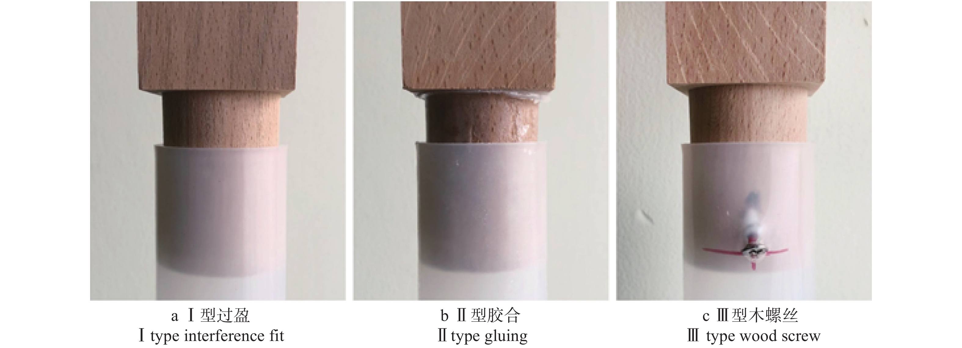
摘要:目的塑料与木材的插接连接是塑料椅类家具中一种常见的节点形式,对节点的配合参量进行优化设计能够有效地提高节点接合强度,从而提升产品的可靠性。方法以PP塑料与榉木圆榫接合构件为例,选择塑料件壁厚、接合长度、过盈配合量为考察因素,以抗拔强度与抗弯强度为评价指标,采用3因素3水平的Box-Behnken响应面设计法,建立接合强度与配合参数之间的数学模型,通过方差分析各因素的显著性及交互作用,同时通过求解拟合方程获得节点的最优配合参量。并在此基础上对过盈、胶合和木螺丝3种不同装配方式的构件节点抗拔力进行对比分析。结果3个因素均对节点的抗拔强度有显著影响,但只有塑料件壁厚和接合长度这两个因素对节点的抗弯强度有显著影响,与过盈配合量无关。直径为40 mm的圆榫塑−木插接节点的最优配合参数为:塑料件壁厚3.2 mm,接合长度50 mm,过盈配合量0.15 mm,对此参数节点进行力学性能试验可获得极限抗拔力2 139.3 N及弯曲载荷1 306.4 N。3种不同装配方式的构件节点抗拔力分别为:过盈装配(Ⅰ型节点)966.5 N < 胶合装配(Ⅱ型节点)1 251.4 N < 木螺丝装配(Ⅲ型节点)1 607.6 N。结论塑−木插接节点的配合参数可以通过响应面法优化设计以获得最佳力学性能,在实际应用中各设计因素在设计域内靠近上限取值较易获得最大接合强度,此外采用木螺丝的装配方式能够大大提高节点的抗拔强度。Abstract:ObjectiveThe insert connection mode between plastic and wood is a common joint form in plastic chair furniture. Optimal design of joint parameters can effectively improve joint strength, thus enhancing the reliability of products.MethodPP plastic and beech jointed by round tenon was put forward as an example, the wall thickness of plastic part, inserting length and interference fit were selected as the observing factors, and the tensile strength and bending strength were taken as evaluation indexes. A three-factor and three-level Box-Behnken response surface design method was used to establish a mathematical model between joint strength and matching parameters. The significance and interaction of each factor were analyzed by analysis of variance, and the optimal assembling and matching parameters of the joint were obtained by solving the regression equation. On this basis, the comparative analysis of the withdrawal forces of joints was carried out between three different assembly forms interference assembly, gluing assembly and wood screw assembly.ResultThe results showed that the three design factors had significant effects on the tensile strength of the joints, but only the wall thickness of plastic parts and the depth of insertion had significant effects on the bending strength of the joints, and had nothing to do with the interference fit. The optimum matching parameters of 40 mm round tenon-wood joints were as follows: the wall thickness of plastic parts was 3.2 mm, the depth of joints was 50 mm, and the interference fit was 0.14 mm. Under this condition, the ultimate withdrawal force and the load of bending of joints were 2 139.3 N and 1 306.4 N. In addition, the withdrawal force of the joints with three different assembly methods was as follows: the interference assembly (type I joint) was 966.5 N < the glued assembly (type II joint) was 1 251.4 N < the wood screw connected assembly (type III joint) was 1 607.6 N.ConclusionThe matching parameters of the plastic-wood insert joint can be optimized by the response surface method to obtain the best mechanical properties. In practical application, it is easy to obtain the maximum joint strength when the design factors are close to the upper limit in the design domain. In addition, the use of wood screws can greatly increase the tensile strength of the joints.
-
土壤有机碳(soil organic carbon,SOC)是植物和微生物生长所必需的物质能量来源,是影响土壤肥力、生产力和养分有效性的关键因素,对土壤理化特性具有重要调节作用[1]。SOC储量分布特征是其长期累积的结果,与土壤剖面的发育密切相关。人工林生态系统具有较强的碳汇和增汇潜能[2],被认为是实现“双碳”目标最经济、最安全的有效途径之一[3]。人工林大面积营建改良了土壤质量,改变了土壤有机质的输入与分解方式,利于SOC贮存和积累[4],人工林土壤碳库库容较大,能维持较稳定的碳储量[5−6]。然而,人工林SOC的贮存受土壤理化性质、植被类型和地形等诸多因素的影响[7−8],关于不同人工林下SOC分布特征尚未达成共识。大量研究基于土壤表层或单一林分,吴慧等[9]研究得出热带山地雨林次生林在0 ~ 50 cm垂直方向上土壤有机碳质量分数随土壤深度增加而减小;王越等[10]通过文献整合分析得出油松(Pinus tabuliformis)林0 ~ 20 cm有机碳储量最高,20 ~ 60 cm稳定且保持较低水平;张智勇等[11]认为陕北黄土区沙棘林有机碳储量优于草地和油松林。据《全球森林评估》报道,我国人工林面积居世界前列[12],人工林生态系统对森林生态系统碳储量增加的贡献较大[13],因此阐明不同人工林SOC储量的分布特征在宏观方向上研究森林碳汇尤为重要。
黄土高原生境脆弱,水土流失严重。随着“退耕还林还草”生态工程的实施,黄土高原植被覆盖大幅增加[14],不同人工林土壤固碳问题逐渐成为研究者们关注的热点问题[15]。土地利用变化的改变增强了土壤碳汇功能[16]。Zhang等[17]研究得出退耕后土壤有机碳储量在0 ~ 20 cm以36.67 g/(m2· a)的速率发生巨大的变化,包玉斌[18]研究了2000—2010年陕北黄土高原退耕年间,其退耕地土壤碳固存总量增加。目前,关于黄土高原SOC储量的研究多集中在大尺度空间分布[19]、单一人工林[20]、模型拟合[21]和浅层土壤(0 ~ 100 cm)[11]。这些研究仅是土地利用前后或退耕后单一林地与草地或农田之间的对比研究,而对于退耕后不同人工林及深层土壤SOC储量的研究较少。相关研究表明,土壤是一个不均匀且不连续的时空变异体[22],其演化过程十分复杂。土壤碳库的分布特征,因缺乏连续、可靠、统一的土壤剖面资料,区域SOC储量实测及代表性数据贫乏[23],存在明显的不确定性[24]。因此,准确评估退耕后小尺度不同人工林SOC储量的分布特征,对森林土壤有机碳库的精确估算以及土壤碳汇研究具有重要意义。
鉴于此,本研究以黄土丘陵区典型同一退耕年限的人工油松林、山杏(Armeniaca sibirica)林、沙棘(Hippophae rhamnoides)林和天然草地0 ~ 200 cm土壤为研究对象,探究不同人工林SOC储量的垂直分布特征,以期为准确计算黄土高原有机碳储量提供数据支撑,为建立黄土高原土壤碳库,优化人工林土壤固碳格局提供理论依据。
1. 研究区概况与研究方法
1.1 研究区概况
研究区位于陕西省吴起县(107°38′57″ ~ 108°32′49″ E,36°33′33″ ~ 37°24′27″ N),海拔高度1 233 ~ 1 809 m,是典型的黄土高原丘陵沟壑区。吴起县地处中温带半湿润—半干旱区域,温带大陆性季风气候特征明显,年均温7.8 ℃,年平均降水量483.4 mm,时空分布不均,主要集中在7—9月,年无霜期146 d。主要土壤类型为黄绵土,结构疏松、持水力低、易侵蚀。自1999年坡耕地转变为林地以来,形成了刺槐(Robinia pseudoacacia)、油松、侧柏(Platycladus orientalis)、山杏、沙棘、柠条(Caragana sinica)、白莲蒿(Artemisia stechmanniana)、达乌里胡枝子(Lespedeza daurica)等以及自然恢复草地为主的乔灌草植物群落,全县林草覆盖率显著增加,生态环境得以改善。
1.2 土壤样品采集与处理
于2020年9月进行样品采集,在研究区选择相同退耕年限的典型人工油松林、山杏林、沙棘林和天然草地,分别布设25 m × 25 m大样方,利用GPS采集地理信息数据,样地基本信息如表1。使用内径6 cm的土钻,在样方内,采用五点采样法,以0 ~ 20 cm、20 ~ 40 cm、40 ~ 60 cm、60 ~ 100 cm、100 ~ 150 cm、150 ~ 200 cm分层采集土壤样品,带回实验室进行分析。待土壤样品风干后,研磨、过筛,进行理化性质测定。土壤密度采用环刀法测定,土壤有机碳采用重铬酸钾稀释热法测定,全氮采用半微量凯式定氮法测定,全磷采用硫酸−高氯酸消煮−钼锑抗比色法定,全碳通过元素分析仪测定,无机碳根据全碳、有机碳之间关系获得,碱解氮采用碱解扩散法测定,速效磷采用钼锑抗比色法测定,土壤粒度组成使用激光粒度分析仪(Mastersize-zer 3000)测定[25]。
表 1 样地基本信息Table 1. Basic information of the sample plots人工林
Plantation海拔
Elevation/m坡度
Gradient/(°)坡向
Aspect平均高度
Average
height/m平均胸径
Average DBH/cm郁闭度或盖度
Crown density or
coverage林下优势种
Dominant understory
species油松 Pinus tabuliformis 1 362.6 20 SFS 8.5 11.3 0.65 MO, LB, ASB 山杏 Armeniaca sibirica 1 459.7 21 SFS 7.3 10.4 0.62 ASB, PS, LB, PC 沙棘 Hippophae rhamnoides 1 389.9 6 NFS 2.9 3.5 0.71 LS, ASW, LB 草地 Grassland 1 376.7 33 SFS 0.86 LB, LS, SC 注:SFS. 阳坡;NFS. 阴坡;MO. 草木犀;LB. 胡枝子;ASB. 白莲蒿;PS. 败酱;PC. 委陵菜;LS. 赖草;ASW. 猪毛蒿;SC. 针茅。Notes: SFS, south-facing slope; NFS, north-facing slope; MO, Melilotus officinalis; LB, Lespedeza bicolor; ASB, Artemisia stechmanniana; PS, Patrinia scabiosaefolia; PC, Potentilla chinensis; LS, Leymus secalinus; ASW, Artemisia scoparia; SC, Stipa capillata. 土壤有机碳储量计算公式为
SOC储量=wSOCi×ρBDi×Di×0.01 式中:SOC储量表示土壤有机碳储量(g/m2),wSOCi表示第i层的土壤有机碳含量(g/kg),ρBDi表示第i层的土壤密度(g/cm3),Di表示第i层的土层厚度。
1.3 数据处理
应用SPSS26.0对数据进行统计分析,采用单因素方差分析(ANOVA)对比不同人工林、不同土层深度有机碳储量之间的差异;应用Origin2018对土壤有机碳储量与土壤理化性质、不同人工林、地形等影响因素之间的关系强弱和作用机理进行PCA分析并绘图;应用R4.2.1对土壤有机碳储量和各环境变量的贡献关系进行冗余分析。
2. 结果与分析
2.1 有机碳储量分布特征
研究区0 ~ 200 cm土层平均SOC储量由大到小为山杏(16.190 g/m2) > 草地(15.403 g/m2) > 沙棘(11.449 g/m2) > 油松(10.188 g/m2)(表2)。不同人工林SOC储量变异系数在10% ~ 30%,为中等程度变异,表现为沙棘(0.219) > 山杏(0.136) > 油松(0.124) > 草地(0.115)。变异系数表征了SOC储量的空间异质性,沙棘的SOC储量空间异质性最大,草地的SOC储量空间异质性最低。
表 2 不同人工林土壤有机碳储量描述统计Table 2. Description statistical characteristics of soil organic carbon stocks content in different plantations人工林
Plantation土层 Soil
layer/cm平均值
Mean value/(g·m−2)最大值
Max. value/(g·m−2)最小值
Min. value/(g·m−2)标准差
Standard deviation变异系数
Variation coefficient占比
Proportion油松
Pinus tabuliformis0 ~ 20 11.658 12.197 10.627 0.893 0.077 0.191 20 ~ 40 7.009 9.253 4.457 2.412 0.344 0.115 40 ~ 60 7.691 8.506 7.267 0.706 0.092 0.126 60 ~ 100 10.246 12.052 8.016 2.051 0.200 0.167 100 ~ 150 13.491 13.844 13.040 0.411 0.030 0.221 150 ~ 200 11.035 11.050 11.010 0.022 0.002 0.180 0 ~ 200 10.188 13.490 7.008 1.082 0.124 山杏
Armeniaca sibirica0 ~ 20 19.049 20.198 16.988 1.789 0.094 0.196 20 ~ 40 13.201 17.450 10.940 3.683 0.279 0.136 40 ~ 60 11.359 12.901 10.199 1.390 0.122 0.117 60 ~ 100 19.106 23.617 15.815 4.041 0.211 0.197 100 ~ 150 20.097 22.132 19.009 1.764 0.088 0.207 150 ~ 200 14.332 14.670 14.033 0.320 0.022 0.147 0 ~ 200 16.190 20.097 11.359 2.184 0.136 沙棘
Hippophae rhamnoides0 ~ 20 19.692 24.417 16.385 4.199 0.214 0.287 20 ~ 40 9.659 13.084 7.616 2.984 0.309 0.141 40 ~ 60 5.912 8.583 4.269 2.333 0.395 0.086 60 ~ 100 8.850 10.196 7.530 1.333 0.151 0.128 100 ~ 150 13.247 15.749 11.861 2.171 0.164 0.193 150 ~ 200 11.333 12.417 10.544 0.971 0.086 0.165 0 ~ 200 11.449 19.691 5.912 2.331 0.219 草地 Grassland 0 ~ 20 19.906 22.351 16.274 3.208 0.161 0.215 20 ~ 40 10.066 11.177 8.118 1.692 0.168 0.109 40 ~ 60 9.256 10.564 8.160 1.216 0.131 0.100 60 ~ 100 14.409 15.494 12.767 1.446 0.100 0.156 100 ~ 150 20.021 20.836 18.609 1.228 0.061 0.217 150 ~ 200 18.760 20.178 17.629 1.299 0.069 0.203 0 ~ 200 15.403 20.021 9.255 1.681 0.115 在不同人工林中(图1),在0~200 cm剖面上SOC储量呈现出山杏(97.145 g/m2) > 草地(92.418 g/m2) > 沙棘(68.695 g/m2) > 油松(61.130 g/m2)的分布格局,山杏的SOC储量与油松、沙棘差异显著(P < 0.05)。人工油松林,山杏林,沙棘林与天然草地0 ~ 60 cm SOC储量占整个剖面的43.11%、44.89%、51.33%、42.45%,表层碳储量高。垂直分布上,油松、山杏、沙棘的SOC储量自表层向下随深度增加变异系数先增大后减小,在20 ~ 40 cm土层变异系数达到最大,草地的SOC储量自表层向下随深度增加变异系数减小。在不同深度土层中,油松的SOC储量与山杏、沙棘、草地在0 ~ 20 cm、20 ~ 40 cm、150 ~ 200 cm土层差异显著(P < 0.05),沙棘的SOC储量与山杏、油松、草地在40 ~ 60 cm、60 ~ 100 cm土层差异显著(P < 0.05),油松、沙棘的SOC储量与山杏、草地在100 ~ 150 cm土层差异显著(P < 0.05)。
![]() 图 1 不同人工林土壤有机碳储量的垂直分布Figure 1. Vertical distribution of soil organic carbon stocks in different plantations
图 1 不同人工林土壤有机碳储量的垂直分布Figure 1. Vertical distribution of soil organic carbon stocks in different plantations2.2 环境因素对典型人工林土壤有机碳储量的影响
典型人工林SOC储量空间变异的主成分分析如下(图2),第一轴和第二轴解释值分别为39.70%和22.70%。第一主成分与部分环境指标的相关系数在0.37以上,其中,PC1与粉粒、黏粒、坡度正相关,与砂粒负相关,第一主成分主要包含了土壤物理性质信息;第二主成分与部分环境指标的相关系数0.5以上,其中PC2与全碳、碱解氮、全氮正相关,主要包含了土壤化学信息,第一和第二主成分反映的信息量占总信息量的62.40%。
![]() 图 2 土壤有机碳储量与土壤环境因子的主成分分析TP. 全磷;TN. 全氮;TC. 全碳;SIC. 土壤无机碳;AP. 速效磷;AN. 碱解氮;Clay. 黏粒;Silt. 粉粒;Sand. 砂粒;ELE. 海拔;SA. 坡向;SG. 坡度。下同。PC1. 第一主成分;PC2. 第二主成分。TP, total phosphorus; TN, total nitrogen; TC, total carbon; SIC, soil inorganic carbon; AP, available phosphorus; AN, alkali-hydrolyzable nitrogen; Clay, clay; Silt, silt; Sand, sand; ELE, elevation; SA, slope aspect; SG, slope gradient. The same below. PC1, the first principal component; PC2, the second principal component.Figure 2. Principal component analysis of soil organic carbon stocks and soil environmental factors
图 2 土壤有机碳储量与土壤环境因子的主成分分析TP. 全磷;TN. 全氮;TC. 全碳;SIC. 土壤无机碳;AP. 速效磷;AN. 碱解氮;Clay. 黏粒;Silt. 粉粒;Sand. 砂粒;ELE. 海拔;SA. 坡向;SG. 坡度。下同。PC1. 第一主成分;PC2. 第二主成分。TP, total phosphorus; TN, total nitrogen; TC, total carbon; SIC, soil inorganic carbon; AP, available phosphorus; AN, alkali-hydrolyzable nitrogen; Clay, clay; Silt, silt; Sand, sand; ELE, elevation; SA, slope aspect; SG, slope gradient. The same below. PC1, the first principal component; PC2, the second principal component.Figure 2. Principal component analysis of soil organic carbon stocks and soil environmental factors2.3 环境因素对土壤剖面有机碳储量垂直分布的影响
不同环境因素对SOC储量垂直变化的贡献度不同(图3)。土壤化学性质、土壤物理性质、地形和植被群落分别对0 ~ 200 cm土壤剖面中SOC储量分布差异的影响约占51.84%、13.58%、30.71%和3.87%。在土壤化学性质中,0 ~ 200 cm SOC储量的变化受全磷影响最大(11.99%),受全氮影响最小(5.64%);在土壤物理性质中,0 ~ 200 cm SOC储量的变化受砂粒影响最大(5.65%),受黏粒影响最小(2.89%);在地形因素中,0 ~ 200 cm SOC储量的变化受海拔影响最大(19.66%),受坡向影响最小(4.97%);植物群落对0 ~ 200 cm SOC储量变化影响较小。
![]() 图 3 土壤化学性质、土壤物理性质、地形和植物群落对土壤有机碳储量变化的相对贡献SCP. 土壤化学性质;SPP. 土壤物理性质;Topo. 地形;PT. 植物群落。SCP, soil chemical property, SPP, soil physical property, Topo, topography, PT, phytocoenosium.Figure 3. Relative contribution of soil chemistry, soil physical properties, topography and phytocoenosium to changes in soil organic carbon stocks
图 3 土壤化学性质、土壤物理性质、地形和植物群落对土壤有机碳储量变化的相对贡献SCP. 土壤化学性质;SPP. 土壤物理性质;Topo. 地形;PT. 植物群落。SCP, soil chemical property, SPP, soil physical property, Topo, topography, PT, phytocoenosium.Figure 3. Relative contribution of soil chemistry, soil physical properties, topography and phytocoenosium to changes in soil organic carbon stocks3. 讨 论
3.1 不同人工林土壤有机碳储量分布差异的对比
本研究发现SOC储量富集在土壤表层,呈现出明显的“表聚性”,这与王文静等[26]的研究结论一致。不同植被群落在土壤浅层聚集了大量的根系和凋落物,凋落物分解产生有机质归还于土壤,通过养分的循环进入土壤[27],因此,大量的有机碳在土壤表层形成和累积。
本研究中,山杏林表现出最优的土壤固碳效益,草地次之,油松林最差,这与李龙波等[28]对乔灌草固碳效益效果的研究结果不一致。植被类型和植被生长间的差异会导致土壤温度、湿度、凋落物数量和根系分泌物等的显著不同[29],进而影响土壤的固碳效益。本研究中草地植被覆盖度高于油松和沙棘林下植被覆盖度(表1),单位面积的植被残体、根系分泌物、枯枝落叶量多,有机质输入量更高,同时,适宜的土壤温度和湿度促进了微生物的生长代谢,提高了植被残体的分解速率,使得草地土壤固碳效率提高。不同人工林中,植物生产力和质量的巨大差异导致SOC储量空间分布的显著差异[30]。且有研究表明,在年平均降水量 < 510 mm区域,草地比灌木和林地积累更多的有机碳[31],本研究区位于黄土丘陵区,年降水量483.4 mm,草地SOC储量高于沙棘和油松。落叶乔木在增加枯落物归还量方面明显优于常绿乔木,这在诸多研究中均有报道[32]。本研究中山杏SOC储量远高于油松,是因为落叶阔叶乔木比常绿针叶乔木产生更多的枯落物凋落量[32],山杏林表层枯落物多,根密度大,不断更替的根系结合不断积累的地表枯落物,不仅改变了土壤腐殖质,也改善了土壤质地,增加了土壤有机碳的积累,因此山杏林具有较高的土壤碳储量,碳汇功能表现较强。
3.2 土壤有机碳储量空间差异的主要影响因素和作用机制
本研究中,不同人工林土壤有机碳储量与黏粒、粉粒和坡度正相关,砂粒与土壤有机碳储量负相关,这阐释了土壤粒径及坡度与土壤有机碳储量之间的关系,这与李顺姬等[33]的研究结果一致。土壤结构是影响有机质分解的主导因素[34],黏粒对土壤有机碳有很好的保护作用,砂质土壤有机碳的矿化更为迅速[33]。当土壤黏粒含量较高时,具有较大的表面积,易形成较多的毛细管,有较强的毛管作用,完整的土壤孔隙为有机碳自表层向下层传输提供了通道,促进深层土壤有机碳固存[35],具有较强的固碳能力。而当土壤砂粒含量较高时,有效土层薄,土壤生物作用弱,土壤有机碳矿化作用较弱,微生物群落质量较低,土壤固碳能力较低。黄土丘陵区“退耕还林还草”工程对土壤机械组成产生一定的影响,使土壤物理性质发生变化。土壤机械组成影响土壤孔隙度、密度,改变土壤的透气性和持水能力,改变植物根系的生长发育及微生物活动条件,进而影响有机碳的储存[36]。坡度显著影响土壤有机碳固存,坡度通过影响水分运移、植被分布及土壤机械组成等间接影响土壤有机碳储量。
本研究中,土壤化学性质对SOC储量的影响较大,全氮、碱解氮、全磷对土壤有机碳储量正向效应显著,阐释了土壤有机碳与土壤养分之间的关系。土壤全氮和碱解氮对土壤有机碳的转化和固存有重要作用。全氮对有机碳储量起正向效应,较高的全氮可以降低凋落物中的碳氮比,避免微生物与植物的“争氮”现象,利于凋落物矿化分解[37],促进土壤有机碳储存。这与王越等[10]研究得出全氮对土壤有机碳呈显著正效应的结果一致。有研究表明,地形显著影响土壤发育、迁移等活动,从而影响土壤碳的输入输出过程[38]。黄土丘陵区水土流失导致了流域内水土资源的重新分配,冗余分析表明,海拔对土壤剖面有机碳储量贮存起主要贡献(图3),通过调控水热条件,进而影响土壤有机碳的积累[39]。
4. 结 论
(1)研究区不同人工林土壤碳储量不同,表现为山杏 > 草地 > 沙棘 > 油松。因此,在黄土高原地区进行人工林营建时,可优先配置山杏林与适宜草种,以增加黄土高原土壤固碳。
(2)研究区不同人工林土壤有机碳储量与土壤机械组成和土壤养分显著相关,黏粒、粉粒、砂粒、全氮、碱解氮是影响黄土丘陵区不同人工林土壤有机碳储量空间分布的主导因子。
(3)研究区人工林土壤有机碳储量在土壤剖面中差异较大,土壤有机碳储量的垂直分布主要受地形的影响。其中,海拔通过影响有机碳的转化与固存对土壤有机碳储量的贮存起主要贡献作用。
-
![]()
图 1 试件尺寸与插接方式
t为塑料件壁厚,单位为mm;d为接合长度,单位为mm;f为过盈配合量,单位为mm;Φ为圆棒直径,单位为mm。t is wall thickness of plastic parts (mm), d is inserting length (mm), f is interference fit (mm), and Φ is diameter of rod (mm).
Figure 1. Size of specimens and method of connection
![]()
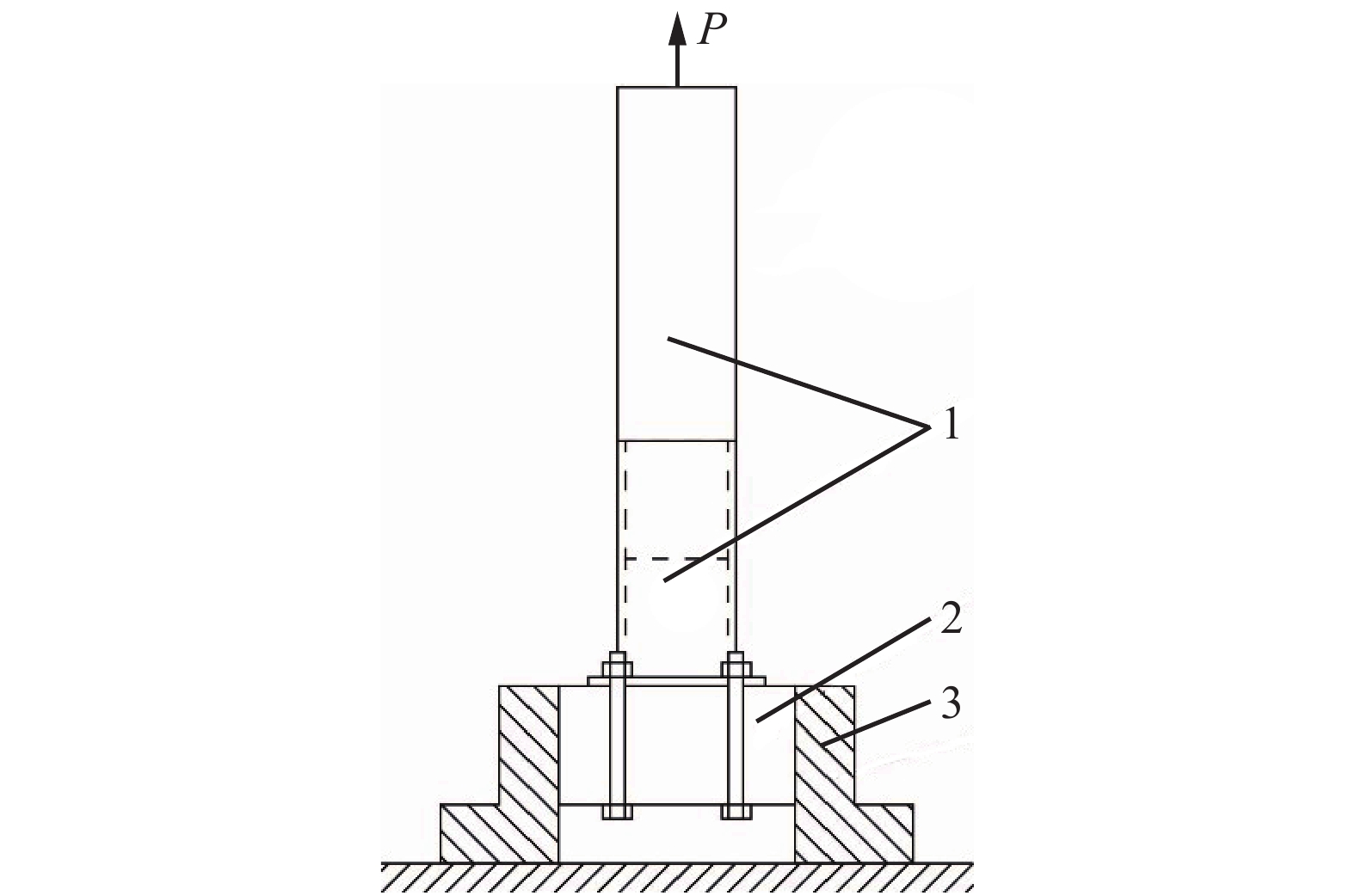
图 2 抗拔性能测试加载方式
1. 试件组件Assembly of specimen;2. 固定支架Fixed support;3. 夹具Fixture;P. 载荷Load/N.
Figure 2. Loading mode of anti-pulling strength experiment
![]()
图 3 抗弯性能测试加载方式
1. 试件组件Assembly of specimen;2. 固定支架Fixed support;3. 夹具Fixture;P. 载荷Load/N.
Figure 3. Loading mode of bending strength experiment
![]()
图 6 抗弯试验中塑−木插接节点的破坏形式
Figure 6. Destroy type of plastic-wood insert joint in bending strength experiment
表 1 试验因子水平设置
Table 1 Experiment factor levels
因素 Factor 水平 Level − 1 0 1 壁厚 Wall thickness of plastic parts (t)/mm 2.4 2.8 3.2 接合长度 Inserting length (d)/mm 30 40 50 配合量 Interference fit (f)/mm 0.05 0.10 0.15  下载: 导出CSV
表 2 响应面分析试验设计及结果
Table 2 Experiment design and results of response surface method
试验号
No.塑料件壁厚
Wall thickness of plastic
parts (t)/mm接合长度
Inserting length (d)/mm配合量
Interference fit (f)/mm抗拔力
Withdrawal force/N弯曲载荷
Bending load/N试验值
Experiment value预测值
Prediction value试验值
Experiment value预测值
Prediction value1 0 0 0 765.7 846.0 1 046.1 1 066.0 2 0 0 0 851.2 846.0 1 065.7 1 066.0 3 0 − 1 − 1 186.6 214.0 743.6 757.8 4 0 1 − 1 445.0 419.0 1 213.2 1 221.7 5 0 − 1 1 1 075.1 1 101.2 829.8 821.3 6 1 − 1 0 447.5 459.1 874.6 868.6 7 1 1 0 992.6 1 057.6 1 305.9 1 305.6 8 0 1 1 1 677.8 1 650.5 1 211.9 1 197.7 9 − 1 0 1 629.8 668.7 935.6 943.8 10 0 0 0 921.1 846.0 1 086.3 1 066.0 11 1 0 − 1 258.9 220.0 1 138.2 1 130.0 12 − 1 1 0 237.2 225.6 1 076.7 1 082.7 13 1 0 1 1 826.5 1 788.9 1 110.6 1 125.1 14 − 1 − 1 0 134.8 69.8 679.2 679.5 15 − 1 0 − 1 81.3 118.9 914.0 899.5
下载: 导出CSV
表 3 抗拔强度方差分析
Table 3 ANOVA of tensile strength
方差来源 Variance source 平方和 Sum of squares df 均方 Mean square F P 显著性 Significance 模型 Model 4.006 × 10⁶ 9 4.451 × 10⁵ 75.34 < 0.000 1 *** 塑料件壁厚 Wall thickness of plastic parts (t) 7.457 × 10⁵ 1 7.457 × 10⁵ 126.21 < 0.000 1 *** 接合长度 Inserting length (d) 2.845 × 10⁵ 1 2.845 × 10⁵ 48.15 0.001 0 ** 配合量 Interference fit (f) 2.244 × 10⁶ 1 2.244 × 10⁶ 379.88 < 0.000 1 *** td 48 995.82 1 48 995.82 8.29 0.034 6 ** tf 2.596 × 10⁵ 1 2.596 × 10⁵ 43.95 0.001 2 ** df 29 635.62 1 29 635.62 5.02 0.075 2 — t2 2.691 × 10⁵ 1 2.691 × 10⁵ 45.55 0.001 1 ** d2 55 849.57 1 55 849.57 9.45 0.027 6 ** f2 55 963.15 1 55 963.15 9.47 0.027 5 ** 残差 Residual 29 541.45 5 5 908.29 失拟项 Lack of fit 17 426.31 3 5 808.77 0.96 0.546 9 纯误差 Pure error 12 115.14 2 6 057.57 总和 Cor total 4.036 × 10⁶ 14 注:拟合度 = 0.992 7;校正拟合度 = 0.979 5;预测拟合度 = 0.924 2;信噪比 = 27.391;变异系数 = 10.95%。“***”表示非常显著;“**”表示显著;“—”表示不显著。Notes: R2 = 0.992 7; Adj R2 = 0.979 5; Pred R2 = 0.924 2; Adeq precision = 27.391; C.V. = 10.95%. “***” means very significant; “**” means significant; “—” means non-significant.
下载: 导出CSV
表 4 抗弯强度方差分析
Table 4 ANOVA of bending strength
方差来源 Variance source 平方和 Sum of squares df 均方 Mean square F P 显著性 Significance 模型 Model 4.544 × 10⁵ 9 50 485.3 127.02 < 0.000 1 *** 塑料件壁厚 Wall thickness of plastic parts (t) 84 830.8 1 84 830.8 213.44 < 0.000 1 *** 接合长度 Inserting length (d) 3.53 × 10⁵ 1 3.53 × 10⁵ 888.19 < 0.000 1 *** 配合量 Interference fit (f) 778.15 1 778.15 1.96 0.220 6 — td 285.61 1 285.61 0.72 0.435 3 — tf 605.16 1 605.16 1.52 0.272 1 — df 1 914.06 1 1 914.06 4.82 0.079 6 — t2 2 994.69 1 2 994.69 7.53 0.040 6 ** d2 10 550.21 1 10 550.21 26.54 0.003 6 ** f2 619.61 1 619.61 1.56 0.267 1 — 残差 Residual 1 987.23 5 397.45 失拟项 Lack of fit 1 179.05 3 393.02 0.97 0.543 0 纯误差 Pure error 808.19 2 404.09 总和 Cor total 1.564 × 10⁵ 14 注:拟合度 = 0.995 6;校正拟合度 = 0.987 8;预测拟合度 = 0.954 7;信噪比 = 38.462;变异系数 = 1.96%。“***”表示非常显著;“**”表示显著;“—”表示不显著。Notes: R2 = 0.995 6; Adj R2 = 0.987 8; Pred R2 = 0.954 7; Adeq precision = 38.462; C.V.= 1.96%. “***” means very significant; “**” means significant; “—” means non-significant.
下载: 导出CSV
表 5 优化方案与结果
Table 5 Schemes and results of optimization
项目 Item 配合参数 Matching parameter/mm 抗拔力
Withdrawal force/N弯曲载荷
Bending load/N塑料件壁厚
Wall thickness of
plastic part (t)/mm接合长度
Inserting length (d)/mm配合量
Interference fit (f)/mm初始值 Initial value 2.8 40 0.10 846.0 1 066.1 优化预测值 Prediction value of optimization 3.2 50 0.15 2 051.2 1 268.3 优化试验值 Experiment value of optimization 3.2 50 0.15 2 139.3 1 306.4
下载: 导出CSV
-
[1] Vassiliou V, Barboutis I. Bending strength of furniture corner joints constructed with insert fittings[J]. Forestry and Wood Technology, 2009, 67: 268−274.
[2] Derikvand M, Ebrahimi G. Strength performance of mortise and loose-tenon furniture joints under uniaxial bending moment[J]. Journal of Forestry Research, 2014, 25(2): 483−486. doi: 10.1007/s11676-014-0479-5
[3] Veysi J, Ghanbar E, Mohsen B. A study of the effects of height and thickness of tenon made out of beech and hornbeam on bending strength of mortise and tenon joint[J]. Iranian Journal of Wood & Paper Science Research, 2010, 25(1): 128−137.
[4] 李敏, 吴智慧, 张继雷. 现代红木家具中直角榫榫卯配合尺寸关系分析[J]. 木材工业, 2016, 30(4):29−32. doi: 10.3969/j.issn.1001-8654.2016.04.007 Li M, Wu Z H, Zhang J L. Tolerance and fit of rectangular mortise and tenon in modern hongmu furniture production[J]. China Wood Industry, 2016, 30(4): 29−32. doi: 10.3969/j.issn.1001-8654.2016.04.007
[5] 陈新义, 刘文金, 孙德林, 等. 梓木构件双圆榫接合性能优化研究[J]. 林产工业, 2014, 41(6):31−33. doi: 10.3969/j.issn.1001-5299.2014.06.008 Chen X Y, Liu W J, Sun D L, et al. Optimization of double dowel of catalpa wood components joint performance[J]. China Forest Products Industry, 2014, 41(6): 31−33. doi: 10.3969/j.issn.1001-5299.2014.06.008
[6] 钟世禄, 关惠元. 椭圆榫过盈配合量与木材密度的关系[J]. 林业科技开发, 2007(2):57−59. doi: 10.3969/j.issn.1000-8101.2007.02.018 Zhong S L, Guan H Y. Relationship between optimal value of interference fit and wood density in oval tenon joint[J]. China Forestry Science and Technology, 2007(2): 57−59. doi: 10.3969/j.issn.1000-8101.2007.02.018
[7] 宋俞成, 朱丽华, 马贞, 等. 梓木家具圆榫接合抗拔强度影响因素试验研究[J]. 林产工业, 2014, 41(3):20−23. doi: 10.3969/j.issn.1001-5299.2014.03.006 Song Y C, Zhu L H, Ma Z, et al. Study on tensile strength influence factors for round tenon joint of catalpa wood furniture[J]. China Forest Products Industry, 2014, 41(3): 20−23. doi: 10.3969/j.issn.1001-5299.2014.03.006
[8] 胡文刚, 白珏, 关惠元. 一种速生材榫接合节点增强方法[J]. 北京林业大学学报, 2017, 39(4):101−107. Hu W G, Bai J, Guan H Y. Investigation on a method of increasing mortise and tenon joint strength of a fast growing wood[J]. Journal of Beijing Forestry University, 2017, 39(4): 101−107.
[9] 陈于书, 刘娜. 桉木多层板插接结构T型构件力学强度的研究[J]. 林产工业, 2017, 44(10):21−26. Chen Y S, Liu N. Study on mechanical strength of eucalyptus multi-layer boards interlocking structure T-shaped specimens[J]. China Forest Products Industry, 2017, 44(10): 21−26.
[10] 李吉庆, 张齐生, 陈礼辉. 竹集成材家具木圆榫接合强度的研究[J]. 西南林业大学学报, 2011, 31(6):74−77. doi: 10.3969/j.issn.2095-1914.2011.06.018 Li J Q, Zhang Q S, Chen L H. Study on joint intensity of wood tenon of laminated bamboo furniture[J]. Journal of Southwest Forestry University, 2011, 31(6): 74−77. doi: 10.3969/j.issn.2095-1914.2011.06.018
[11] 胡文刚, 关惠元. 基于摩擦特性的榫接合节点抗拔力研究[J]. 林业工程学报, 2017, 2(4):158−162. Hu W G, Guan H Y. Investigation on withdrawl force of mortise and tenon joint based on friction properties[J]. Journal of Forestry Engineering, 2017, 2(4): 158−162.
[12] 关惠元. 现代家具结构讲座(第六讲): 非木质家具结构[J]. 家具, 2007(6):50−59. Guan H Y. Lecture on modern furniture structure (lecture 6): non-wood furniture structure[J]. Furniture, 2007(6): 50−59.
[13] 王安正, 关惠元. 基于响应面法的塑料椅板式构件优化设计研究[J]. 塑料工业, 2019, 47(1):69−73. doi: 10.3969/j.issn.1005-5770.2019.01.015 Wang A Z, Guan H Y. Study on the optimization of flat plastic chair component based on the response surface methodology[J]. China Plastic Industry, 2019, 47(1): 69−73. doi: 10.3969/j.issn.1005-5770.2019.01.015


计量
- 文章访问数: 1675
- HTML全文浏览量: 773
- PDF下载量: 33
