雌雄异株植物簇毛槭繁殖代价延迟效应研究

赵海艳; 宋子龙; 徐萌; 黄云浩; 张新娜; 王娟

doi:10.13332/j.1000-1522.20180360

雌雄异株植物簇毛槭繁殖代价延迟效应研究

1.
北京林业大学森林资源与生态系统过程北京市重点实验室，北京 100083
2.
吉林省蛟河林业实验区管理局，吉林蛟河 132517

基金项目: 国家自然科学基金（31600480）

详细信息

作者简介:
赵海艳。主要研究方向：繁殖生态学。Email：zhaohaiyan_2016@163.com　地址：100083北京市海淀区清华东路35号北京林业大学林学院

责任作者:
王娟，副教授。主要研究方向：繁殖生态学。Email：wangjuan@bjfu.edu.cn　地址：同上

中图分类号: S718.3; Q945.5; S792.35
计量
- 文章访问数: 2486
- HTML全文浏览量: 890
- PDF下载量: 71
出版历程
- 收稿日期: 2018-11-28
- 修回日期: 2018-12-30
- 网络出版日期: 2019-06-14
- 发布日期: 2019-07-31

Delayed effects of reproductive costs in dioecious species Acer barbinerve

1.
Key Laboratory for Forest Resources & Ecosystem Processes of Beijing, Beijing Forestry University, Beijing 100083, China
2.
Administration Bureau for Jiaohe Forestry Experimental Area, Jiaohe, 132517, Jilin, China

摘要

摘要:
目的植物将大部分资源用于繁殖活动时必将导致其对生长发育等其他功能的资源投入下降，生活史理论把这种现象称为繁殖代价。植物繁殖代价主要体现为当年繁殖资源投入与当年营养生长资源投入之间的权衡，以及当年繁殖资源投入与未来生长发育资源投入之间的权衡，这意味着植物的繁殖代价可能存在着一定的延迟效应。本文利用雌雄异株植物雌雄功能分离的属性，验证吉林蛟河针阔混交林中簇毛槭是否存在繁殖代价的延迟效应。
方法2012年选取簇毛槭雌雄各90株，将不同性别植株分成3个处理组（A为对照组，B为摘除花朵即开花不结实组，C为摘除花蕾组）进行试验操作。2013年和2017年跟踪调查不同处理组中簇毛槭繁殖及生长状况。利用双因素方差分析检验不同处理方式下雌雄植株的1年生枝条长度和叶片生物量的差异显著性。
结果2013年花期，在1年生枝条水平和2级侧枝水平上1年生枝条长度顺序为C组 > B组 > A组。其中雌株的B组和C组显著大于A组，雄株的处理组间差异显著。2013年花期，在1年生枝条水平和2级侧枝水平上雌株的叶片生物量顺序为C组 > B组 > A组；其中B组和C组显著大于A组。2017年花期，在1年生枝条水平雄株的叶片生物量顺序为C组 > B组 > A组，其中C组显著大于A组。
结论构件水平影响着繁殖代价延迟效应的检测结果；雌雄异株树种簇毛槭的繁殖代价的延迟效应在营养器官上的表现具有性别和养分分配差异；繁殖代价延迟效应持续表现时间也具有性别差异。
- 繁殖代价 /
- 雌雄异株 /
- 簇毛槭 /
- 延迟效应
Abstract:
ObjectivePlant resource allocation is limited such that an increase reproduction incurs a reduction in other functions, quantified as reduced current growth, development or survival. This phenomenon is called reproductive cost based on the theory of life history evolution. Sometimes the cost of reproduction can be shown in the trade-off between the cost of reproduction in the current year and the growth in the future, suggesting that the reproductive cost has a delayed effect. Dioecious plant Acer barbinerve, in which reproductive functions are separated into two distinct sexual forms, is especially suitable for studying the delayed effect of reproductive cost in a coniferous and broadleaved mixed forest in Jiaohe, Jilin Province of northeastern China.
MethodTo explore the delayed effect of reproductive cost, we selected 90 female and 90 male individuals with no significant difference in size of dioecious species Acer barbinerve in 2012. The individuals of each sex were divided into three treatments (A, control; B, removing flower called flowers only without fruits; C, removing flower bud). We investigated the reproduction and growth of Acer barbinerve in different treatments in 2013 and 2017. Two-way ANOVAs was performed to test the difference of length of new shoot and foliage biomass for each sex under different treatments.
ResultIn flowering time in 2013, the sequence of length of new shoot was group C > group B > group A at shoot and branch level, in which the difference of group B and group C with group A was significantly separated. The differences under different treatments of male were significant. In flowering times in 2013, the foliage biomass of female was group C > group B > group A at shoot and branch level. The leaf biomass of male plants in the flowering times at shoot level of 2017 was C > B > A, in which group C was significantly larger than group A.
ConclusionThe delayed effect of reproductive cost of dioecy Acer barbinerve was influenced by module level and showed sexual difference in different vegetative organs and nutrient distribution, also had gender differences in the duration.
- reproductive cost /
- dioecy /
- Acer barbinerve /
- delayed effect

HTML全文

森林是陆地生态系统的主要碳储存库，在全球碳循环和生态系统服务中发挥着重要作用^[1-2]。及时精确地估算森林碳储量有助于评估森林碳库的现状及变化速率，为应对气候变化制定政策提供重要依据。因此，森林生物量的精确快速估测，特别是大尺度范围的估测^[3]，对及时掌握森林的生态价值，优化森林经营方案具有重要意义。

森林生物量的估算方法主要有实地测量和遥感提取两种方法^[4]。传统的实地调查测量方法能提供关于森林组成和结构的详细资料，但耗费大量的人力、物力和财力，并且不适用于大范围森林生物量估算和动态变化监测^[5]。随着遥感技术的快速发展，包括被动光学成像^[6-7]、合成孔径雷达（synthetic aperture radar，SAR）^[8-10]和激光扫描（light detection and ranging，LiDAR）^[11-12]遥感数据已经应用于森林生物量估算，而且不同类型的遥感变量具有各自的优势。SAR不受云层的影响，同时对树冠有一定的穿透能力，波长越长穿透能力越强^[13-14]。研究表明，与C波段和X波段相比，L波段和P波段更适合用于估算森林生物量^[15-18]。然而，目前在轨运行的L波段星载SAR数据只有ALOS PALSAR-2，机载SAR数据获取成本昂贵，因此目前满足条件的SAR数据源不是很丰富。此外，SAR数据受地形影响很大，阴影、叠掩和收缩等现象严重影响数据质量。这些因素都限制了利用SAR进行大区域尤其是山地区域森林生物量的估测^[19-20]。LiDAR可以反演得到高精度的森林结构参数，解决生物量饱和的问题，提高森林生物量的估算精度^[20]。不过机载LiDAR数据作为主要的LiDAR数据源，数据采集成本高，同时很难在点云密度、数据分析精度和分析效率之间取得平衡，因此在大范围森林参数反演中的应用受到限制^[21]。

与SAR、LiDAR相比，光学遥感数据源从低空间分辨率到高空间分辨率，从多光谱到高光谱，可以提供丰富的光谱信息、植被指数信息和空间特征信息等^[22-23]。由欧空局发射的Sentinel-2A卫星比Landsat、MODIS等其他开放数据源具有更高的空间分辨率和时间分辨率，它包含的3个红边波段、2个近红外波段和2个短波红外波段与植被密切相关^[24]，更有利于森林资源监测。多数植被指数是由各个波段组合而成，蕴含十分丰富的植被信息^[25]，郑阳等^[26]提取Sentinel-2A数据的17种宽波段植被指数，特别是红边指数，并从中筛选出与生物量相关性高的植被指数构建了冬小麦地上生物量估算模型，提高了生物量的估算精度；曹霖等^[27]以Sentinel-2A为数据源，结合光谱反射率、植被指数和地形因子等信息，采用多元线性回归等算法构建了吉林中东部森林蓄积量的反演模型；Santa Pandit等^[28]针对难以到达的森林内部利用Sentinel-2中的植被指数经过随机森林算法的筛选，推算出适用于亚热带地区的一种生物量估算模型；陈瑜云^[29]结合多个时期的影像的光谱波段和植被指数等信息，采用随机森林方法得到了南方毛竹林的地上生物量观测模型；利用Sentinel-2A红边波段的森林生物量估测相关研究^{[27, 30-32]}，证明了红边波段以及生物物理参数对生物量的估算具有积极意义。然而，在林业遥感应用领域，对基于Sentinel-2A获取的各类信息，包括波段信息、植被指数信息和生物物理参数信息在进行生物量估算时的能力的对比研究还较少。因此，需要进行更深入的研究来评估新一代光学卫星图像在森林生物量反演上的表现。

本研究以Sentinel-2A为数据源，探究光谱波段、植被指数和生物物理参数估算针叶林地上生物量的能力，以及高程因子对温带针叶林地上生物量的影响，建立不同的针叶林地上生物量估算模型，分析不同类型特征在针叶林地上生物量估算中的潜力。同时反演得到整个旺业甸林场的针叶林地上生物量，为了解内蒙古东北地区的碳储量提供数据支撑。

1. 研究区概况

本文研究区设置在内蒙古自治区赤峰市喀喇沁旗西南部的旺业甸林场（118°09′ ~ 118°30′ E，41°21′ ~ 41°39′ N）（图1）。林场总面积近500 km²，以山地为主，南北约28.1 km，东西约30.3 km，海拔分布在800 ~ 1 890 m之间。该研究区属于温带大陆性季风气候，冬季寒冷干燥，夏季温暖多雨，年平均气温3.5 ~ 7.0 ℃，年均降水量为300 ~ 500 mm。林场以人工林为主，包括针叶林和阔叶林，其中针叶树种有落叶松（Larix gmelinii）、油松（Pinus tabuliformis）、红松（Pinus koraiensis ）和樟子松（Pinus sylvestris）等，阔叶树种有白桦（Betula platyphylla）、山杨（Populus davidiana）和榆树（Ulmus pumila）等。其中，油松和落叶松是该林场针叶林的优势树种，面积分别为128.05 和 76.27 km²，占针叶林总面积的61.85%和36.84%。因此，估算油松和落叶松两个树种的地上生物量（aboveground biomass，AGB）对于更好地理解林场针叶林的碳动态具有重要意义。

图 1 研究区位置及调查样地分布图

Figure 1. Location of study area and distribution of surveying sample plots

下载: 全尺寸图片幻灯片

2. 研究方法

2.1 地面数据采集与生物量计算

野外数据采集工作于2017年9月在旺业甸林场开展。林场内针叶林树种以落叶松和油松为主，覆盖范围大，具有代表性，红松、樟子松等其他针叶树种多以十分稀疏的混交形式分布，且面积较小，很难开展样地数据采集，因此本研究以油松和落叶松作为针叶林代表树种反演针叶林的地上生物量。设置正方形样地大小为25 m × 25 m，依据远离道路、均匀分布、覆盖不同林龄的原则，共获取81块具有代表性的针叶纯林样地，其中落叶松41块，油松40块。首先，利用实时差分定位仪（real-time kinematic, RTK）对样地的角点和中心点进行精确定位；其次，记录样地的环境因子，如海拔、坡度、坡向、坡位、林龄和郁闭度等；最后，对样地内胸径大于5 cm的树木进行每木检尺，记录胸径、树高和枝下高等信息。

本研究采用异速生长模型计算得到的样地森林生物量作为建模和验证数据。先利用样地调查数据计算样地内每棵树的生物量，再将所有树的生物量相加得到样地生物量。根据当地林业统计方式，落叶松和油松的地上生物量分别计算，计算模型^[33]如表1所示。

表 1 落叶松、油松的生物量计算模型

Table 1. Biomass calculating models of Larix gmelinii and Pinus tabuliformis

树种(组) Tree species (group)	生物量模型和参数 Biomass model and parameter
落叶松 Larix gmelinii	${W}_{{\rm{r}}}=0.0462\;38{\left({D}^{2}H\right)}^{0.905\;002}$
油松 Pinus tabuliformis	${W}_{{\rm{S}}}=0.0276\;36{\left({D}^{2}H\right)}^{0.990\;5};$ ${W}_{{\rm{B}}}=0.00913\;13{\left({D}^{2}H\right)}^{0.982};$ ${W}_{{\rm{L}}}=0.00457\;55{\left({D}^{2}H\right)}^{0.989\;4};$ ${W}_{{\rm{r}}}={W}_{{\rm{S}}}+{W}_{{\rm{B}}}+{W}_{{\rm{L}}}$
注： ${W}_{{\rm{S}}}$ 、 ${W}_{{\rm{B}}}$ 、 ${W}_{{\rm{L}}}$ 、 ${W}_{{\rm{r}}}$ 分别为树干生物量、树枝生物量、树叶生物量、地上部分总生物量，t/hm²；D为胸径，cm；H为树高，m。Notes: ${W}_{{\rm{S}}}$ , ${W}_{{\rm{B}}}$ , ${W}_{{\rm{L}}}$ , ${W}_{{\rm{r}}}$ indicate stem biomass, branch biomass, leaf biomass, total aboveground biomass, respectively, t/ha; D is DBH, cm; H is tree height, m.

下载: 导出CSV

| 显示表格

2.2 Sentinel-2A数据

Sentinel-2是一项宽扫描、高分辨率、多光谱成像的对地观测任务，由两颗卫星（Sentinel-2A和Sentinel-2B）组成，可用于对植被、土壤和水的监测研究。欧洲航天局在2015年发射了Sentinel-2A卫星，2017年发射了Sentinel-2B卫星，这两颗卫星每5天可完成一次对地球赤道地区的完整成像。Sentinel-2A卫星携带一枚多光谱成像仪，覆盖13个光谱波段，其中4个波段空间分辨率为10 m，6个波段空间分辨率为20 m，3个波段空间分辨率为60 m。本研究采用空间分辨率为10和20 m的波段。

本研究从哥白尼科学数据中心（Copernicus Scientific Data Hub，CSDB（https://scihub.copernicus.eu/））下载两景2017年9月22日的Sentinel-2A Level-1C影像。利用Sen2Cor大气校正处理器（2.5.5版本）进行大气校正得到Level-2A大气底层反射率数据。采用C模型进行地形校正，减小地形的影响。最后，所有波段影像重采样到10 m分辨率。

2.3 数字高程模型DEM数据

在地理空间数据云（http://www.gscloud.cn）上下载90 m分辨率的DEM数据。将数据投影转换成与Sentinel-2A相同（WGS_1984_UTM_zone_50N），提取高程信息，重采样到10 m分辨率。

2.4 分类辅助数据

林场的森林类型（针叶林、阔叶林和混交林）分类图以旺业甸实验林场2018年的小班数据为依据生成。小班数据包括森林类型、林龄组、立地类型等属性。对森林类型属性进行筛选，选择所有针叶林树种，生成旺业甸实验林场针叶林分布图。

2.5 变量提取

本研究从Sentinel-2A获取10个波段光谱信息、20个植被指数和5个生物物理参数，从研究区DEM获取高程信息（表2）。将基于PROSPECT模型得到的植物叶片反射率和透射率输入斜叶反射模型（scattering by arbitrarily inclined leaves，SAIL）中得到冠层反射率，再利用L2B反射率图像计算得到生物物理参数。计算得到的生物物理参数包括叶面积指数（LAI）、植被覆盖度（FVC）、叶片叶绿素含量（Cab）、冠层含水量（Cwc）和有效光合吸收辐射度（FAPAR）。不同阶段森林的生长状态可以反映在波段信息中，而且生长所需的水分、光照和温度等自然因素也会随着森林的立地情况发生改变，因此遥感数据中提取的直接变量与森林地上生物量关系密切；植被指数是由波段信息经过不同组合得到的，提供了特有的冠层光谱信息，可能作为波段信息的替代信息反演森林地上生物量；生物物理参数提供了有关生物物理特征的信息，这些参数可以间接反映出植物的生长状况^[34]；另外，有研究表明，地形变量是反映植被分布和生长环境的重要参数，有助于提高生物量估算的精度^[35-37]。

表 2 生态变量列表

Table 2. List of ecological variables

数据源 Data source	类别 Type	变量名称 Variable name	属性 Attribute	公式 Formula
Sentinel-2A	波段信息 Band information	B2	蓝色 Blue (波长 Wavelength (WL), WL = 490 nm)
		B3	绿色 Green (WL = 560 nm)
		B4	红色 Red (WL = 665 nm)
		B5	红边波段 Red edge band (WL = 705 nm)
		B6	红边波段 Red edge band (WL = 749 nm)
		B7	红边波段 Red edge band (WL = 783 nm)
		B8	近红外 Near infrared (WL = 842 nm)
		B8a	近红外 Near infrared (WL = 865 nm)
		B11	短波红外 Shortwave infrared (WL = 1 610 nm)
		B12	短波红外 Shortwave infrared (WL = 2 190 nm)
	植被指数 Vegetation index	RVI	比值植被指数 Ratio vegetation index	B8/B4
		DVI	差值植被指数 Difference vegetation index	B8 − B4
		WDVI	权重差值植被指数 Weighted difference vegetation index	${\rm{B}}8 - 0.5\times {\rm{B}}4$
		IPVI	红外植被指数 Infrared vegetation index	B8/(B8 + B4)
		PVI	垂直植被指数 Perpendicular vegetation index	$\sin (45^\circ)\times {\rm{B}}8 - \cos (45^\circ)\times {\rm{B}}4$
		NDVI	归一化差值植被指数 Normalized difference vegetation index	(B8 − B4)/(B8 + B4)
		NDVI45	B4和B5归一化差值植被指数 NDVI with band4 and band5	(B5 − B4)/(B5 + B4)
		GNDVI	绿波归一化差值植被指数 NDVI of green band	(B7 − B3)/(B7 + B3)
		IRECI	反红边叶绿素指数 Inverted red edge chlorophyll index	(B7 − B4)/(B5/B6)
		SAVI	土壤调节植被指数 Soil adjusted vegetation index	1.5 × (B8 − B4)/8 × (B8 + B4 + 0.5)
		TSAVI	转化土壤调节植被指数 Transformed soil adjusted vegetation index	0.5 × (B8 − 0.5 × B4 − 0.5)/(0.5 × B8 + B4 − 0.15)
		MSAVI	修正型土壤调节植被指数 Modified soil adjusted vegetation index	$\begin{array}{l}\left ( {2 - {\rm{NDVI}} \times {\rm{WDVI}}} \right) \times \left ( {{\rm{B}}8 - {\rm{B}}4} \right)/ \\8 \times \left ( {{\rm{B}}8 + {\rm{B}}4 + 1 - {\rm{NDVI}} \times {\rm{WDVI}}} \right)\end{array}$
		MSAVI2	二次修正型土壤调节植被指数 Secondly modified soil adjusted vegetation index	$0.5 \times \left[ {2 \times \left ( {{\rm{B}}8{\rm{}} + {\rm{}}1} \right) - \sqrt {{{\left ( {2 \times {\rm{B}}8 + 1} \right)}^2} - 8 \times \left ( {{\rm{B}}8 - {\rm{B}}4} \right)} } \right]$
		ARVI	大气阻抗植被指数 Atmospherically resistant vegetation index	${\rm{B}}8- (2\times {\rm{B}}4-{\rm{B}}2)/{\rm{B}}8+ (2\times {\rm{B}}4-{\rm{B}}2)$
		PSSRa	特定色素简单比值植被指数 Pigment specific simple ratio chlorophyll index	B7/B4
		MTCI	Meris陆地叶绿素指数 Meris terrestrial chlorophyll index	(B6 − B5)/(B5 − B4)
		MCARI	修正型叶绿素吸收比植指数 Modified chlorophyll absorption ratio index	$\left[\left ({\rm{B}}5-{\rm{B}}4\right)-0.2\times ({\rm{B}}5-{\rm{B}}3)\right]\times ({\rm{B}}5-{\rm{B}}4)$
		S2REP	“哨兵2号”红边位置指数 Sentinel-2 red edge position index	$705+35\times \left[\dfrac{\left ({\rm{B}}4+{\rm{B}}7\right)}{2}-{\rm{B}}5\right]\times ({\rm{B}}6-{\rm{B}}5)$
		REIP	红边感染点指数 Red edge infection point index	$700+40\times \left[\dfrac{\left ({\rm{B}}4+{\rm{B}}7\right)}{2}-{\rm{B}}5\right]/ ({\rm{B}}6-{\rm{B}}5)$
		GEMI	全球环境监测指数 Global environmental monitoring index	$\begin{array}{l}{\rm{eta}} \times \left ( {1 - 0.25 \times {\rm{eta}}} \right) - \dfrac{{{\rm{B}}4 - 0.125}}{{1 - {\rm{B}}4}}, \\{\rm{eta}}= [ 2 \times \left ( {{\rm{B}}8{\rm{A}} - {\rm{B}}4} \right) + 1.5 \times {\rm{B}}8{\rm{A}} + 0.5 \times {\rm{B}}4 ]/\\ \left ( {{\rm{B}}8{\rm{A}} + {\rm{B}}4 + 0.5} \right)\end{array}$
	生物物理参数 Biophysical parameter	LAI	叶面积指数 Leaf area index
		FVC	植被覆盖度 Vegetation coverage
		FAPAR	有效光合吸收辐射度 Effective photosynthetically absorbed radiance
		Cab	叶绿素含量 Chlorophyll content
		Cwc	冠层水分含量 Canopy water content
SRTM DEM	地形指数 Topographic index	H	高程 Elevation

下载: 导出CSV

| 显示表格

2.6 生物量估算模型的建立与评价

尽管目前像机器学习方法之类的许多计算方法已开始用于对森林生物量的估测，凭借着良好的预测能力，构建多元回归模型仍然是最常用的方法。本文采用多元逐步回归的方法，以基于影像提取的变量为自变量，以实测的样地生物量为因变量，构建针叶林AGB估算模型。

将基于Sentinel-2A获取的变量分成4组建立针叶林AGB估算模型：（1）只有10个光谱反射率变量；（2）只有20个植被指数变量；（3）只有5个生物物理参数变量；（4）前3组筛选出的所有变量（图2）。首先，对每组变量进行皮尔逊相关性分析，选择出与AGB呈显著相关的变量；其次，采用多元逐步回归的方法建立方程，选择出既与AGB相关性强又与其他变量不存在自相关的最佳变量组合，分析各类型变量对针叶林AGB的影响。同时，我们用DEM的高程数据作为补充变量，加入各组已建好的方程中，评估高程是否能改善针叶林AGB的预测效果。

图 2 技术路线图

Figure 2. Technology flowchart

下载: 全尺寸图片幻灯片

本研究将81个样地数据按照训练样本和验证样本7∶3划分，得到61个训练样本和20个验证样本。利用训练样本结合皮尔逊相关性分析筛选出的变量建立模型，建模过程中每引入一个自变量或剔除一个自变量前后都进行假设检验，直至既没有自变量能够进入方程，也没有自变量从方程中剔除为止。为了评估模型的性能，利用验证样本对模型进行有效性检验，采用均方根误差（root mean square error，RMSE）、相对均方根误差（relative root mean square error，rRMSE）以及平均绝对百分误差（mean absolute percentage error，MAPE）来验证并评价模型的预测能力^[36]。

${\rm{RMSE}} = \sqrt {\frac{1}{n}\sum\nolimits_1^n {{\left( {{Y} - {{\hat Y}}} \right)}^2}}$

(1)

${\rm{rRMSE}} = \frac{{{\rm{RMSE}}}}{{{{\bar Y}}}} \times 100\%$

(2)

${\rm{MAPE}} = \frac{1}{n}\sum\nolimits_1^n \left| {\frac{{{Y} - {{\hat Y}}}}{{{{\hat Y}}}} \times 100\% } \right|$

(3)

式中：Y代表预测生物量， ${\hat{Y}}$ 代表实测生物量， ${\bar{Y}}$ 代表实测生物量的均值，n为样本量。

3. 结果与分析

3.1 Sentinel-2A数据与生物量的关系

表3为各组变量与针叶林生物量之间的皮尔逊相关性分析结果。可以看出，10个波段信息与针叶林地上生物量之间呈显著相关（P < 0.01），说明波段信息与针叶林地上生物量之间关系密切，因此10个波段信息参与下一步利用多元逐步回归方法建立估算模型；利用20个植被指数与针叶林地上生物量的皮尔逊相关性分析结果可以将相关性较差的比值植被指数（ratio vegetation index，DVI）、转化土壤调节植被指数（transformed soil adjusted vegetation index，TSAVI）、二次修正型土壤调节植被指数（second modified soil adjusted vegetation index，MSAVI2）、“哨兵2号”红边位置指数（sentinel-2 red-edge position index，S2REP）和全球环境监测指数（global environmental monitoring index，GEMI）剔除，不参与后续多元逐步回归建模；5个生物物理参数中，叶面积指数（LAI）、有效光合吸收辐射度（FAPAR）、叶绿素含量（Cab）和冠层水分含量（Cwc）与针叶林地上生物量之间相关性更强；另外，高程信息与针叶林地上生物量之间显著性水平也达到0.01。

表 3 变量与地上生物量之间的相关性分析

Table 3. Correlation analysis of aboveground biomass and variables

变量 Variable	相关系数 Correlation coefficient	变量 Variable	相关系数 Correlation coefficient	变量 Variable	相关系数 Correlation coefficient	变量 Variable	相关系数 Correlation coefficient
B2	−0.590**	RVI	0.748**	TSAVI	−0.092	LAI	0.527**
B3	−0.588**	DVI	−0.352*	MSAVI	−0.418**	FVC	−0.123
B4	−0.526**	WDVI	−0.405**	MSAVI2	−0.267	FAPAR	0.528**
B5	−0.572**	IPVI	0.582**	ARVI	−0.534**	Cab	0.459**
B6	−0.489**	PVI	0.462**	PSSRa	0.757**	Cwc	0.643**
B7	−0.417**	NDVI	0.582**	MTCI	0.700**	H	0.425**
B8	−0.442**	NDVI45	0.569**	MCARI	−0.502**
B8a	−0.444**	GNDVI	0.685**	S2REP	0.105
B11	−0.582**	IRECI	0.589**	REIP	0.620**
B12	−0.585**	SAVI	−0.393**	GEMI	−0.311*
注：代表显著性水平为0.05，代表显著性水平为0.01。下同。Notes: means the significance level is 0.05 and ** is 0.01. Same as below.

下载: 导出CSV

| 显示表格

表4为分4组建立针叶林生物量模型的评价结果。可以看出，采用多元逐步回归方法所建立的估算模型的R²在0.465到0.765之间，不同类型变量建立的模型生物量估算效果有较大差异。从10个波段反射率中采用逐步多元回归方法获得以B4和B12为自变量的针叶林AGB估算模型；在20个植被指数中进行回归分析筛选，PSSRa和AVRI被筛选为最终的预测变量；得到的5个生物物理参数中，筛选出LAI、FAPAR和Cwc3个变量参与建模；在第4组中，将以前3组建模过程筛选出的全部变量为基础建立模型，最终得到了以PSSRa、AVRI和Cwc为自变量的针叶林AGB 估算方程。在建立的4组AGB模型中，高程变量的加入都将原来的模型决定系数（R²）提高了0.1左右，说明高程信息对于提高AGB的预测精度具有积极意义。

表 4 模型评价结果

Table 4. Evaluation results of models

数据源 Data source	类别 Type	预测变量 Predictive variable	决定系数 R²	显著性 Significance	均方根误差/(t·hm⁻²) RMSE/(t·ha⁻¹)
Sentinel-2A	波段信息 Band information	B4 + B12	0.465	< 0.01	49.27
	波段信息 Band information	B4 + B12 + H	0.523	< 0.01	47.33
	植被指数 Vegetation index	PSSRa + AVRI	0.601	< 0.01	44.08
	植被指数 Vegetation index	PSSRa + AVRI + H	0.682	< 0.01	41.14
	生物物理参数 Biophysical parameter	LAI + FAPAR + Cwc	0.506	< 0.01	46.31
	生物物理参数 Biophysical parameter	LAI + FAPAR + Cwc + H	0.604	< 0.01	44.62
	不分组 No grouping	PSSRa + AVRI + Cwc	0.673	< 0.01	41.84
	不分组 No grouping	PSSRa + AVRI + Cwc + H	0.765	< 0.01	39.49

下载: 导出CSV

| 显示表格

比较分析4组针叶林AGB估算模型，3类特征变量筛选后的变量建立的方程R²最高，其次是基于植被指数和生物物理参数所建的方程，基于波段反射率建立的方程R²最低。高程变量的加入对基于生物物理参数建立的模型效果改善最多，对于波段信息建立的模型虽有改善但变化不大。

3.2 生物量预测及评价

利用4个生物量预测组中的最佳模型（最高R²和最低的RMSE）得到的模型开展进一步分析并估算绘制研究区域内针叶林AGB，具体模型如表5所示。

表 5 模型精度评价表

Table 5. Evaluation of model accuracy

类别 Type	模型方程 Model equation	均方根误差/(t·hm⁻²) RMSE/(t·ha⁻¹)	相对均方根误差 Relative root mean square error (rRMSE)/%	平均绝对百分误差 Mean absolute percentage error/%
波段信息 Band information	Y = −104.388 − 47 558.708 × B12 + 20 487 × B4 + 0.255 × H	47.33	33.97	33.03
植被指数 Vegetation index	Y = 214.919 + 22.950 × PSSRa − 735.420 × AVRI + 0.176 × H	41.14	29.53	25.98
生物物理参数 Biophysical parameter	Y = −1 059.178 + 8 097.090 × Cwc − 1 219.432 × LAI + 4 037.249 × FAPAR + 0.441 × H	44.62	32.03	29.73
不分组 No grouping	Y = 147.724 + 19.581 × PSSRa − 770.512 × AVRI + 1 593.239 × Cwc + 0.230 × H	39.49	28.35	27.96

下载: 导出CSV

| 显示表格

表5为4个模型进行精度评价的结果，RMSE在39.49到47.33 t/hm²之间，rRMSE在28.35%到33.97%之间，MAPE在25.98%到33.03%之间。可以看出，模型表现最好的是多种类型变量相结合的第4组，而单一变量类型估算中，植被指数的估算效果最好，波段反射率变量的估算效果最差。

图3是对4个模型利用预测生物量与实测生物量绘制散点图和残差图。4个模型预测值与实测值拟合效果差别较大，但整体呈现出在低生物量处存在高估，在高生物量处存在低估的现象。通过比较分析4个模型的残差图发现，相比于3组单一类型变量的估算，基于多类型变量的第4组模型在0 ~ 150 t/hm²区间的残差明显减小，尤其是0 ~ 100 t/hm²区间。在高于150 t/hm²的区间，由于受到数据饱和的影响，生物量都呈现出低估的现象，第四组模型效果相对较好，残差都低于60 t/hm²。

图 3 预估生物量与实测生物量的散点图与残差图

Figure 3. Scatter plots and residual plots of predicted and measured biomass

下载: 全尺寸图片幻灯片

本文利用预估效果最好的模型4对整个旺业甸林场的针叶林进行生物量反演。利用2018年更新的林场小班图为基础，通过属性筛选得到针叶林的范围，在此基础上反演得到旺业甸林场的针叶林生物量反演图（图4）。反演结果显示，旺业甸林场西北部及中部区域生物量较低，东部及南部地区生物量较高，与实际情况相符，反演效果较好。

图 4 旺业甸林场针叶林生物量反演分布图

Figure 4. Biomass inversion distribution of coniferous forest in Wangyedian Forest Farm

下载: 全尺寸图片幻灯片

4. 讨　　论

在基于Sentinel-2A获取的3类特征变量中，利用植被指数构建的模型效果好于基于波段反射率信息和生物物理参数所建的模型。在光谱反射率特征组中，针叶林AGB估算模型选择了红光波段（B4）和短波红外波段（B12）的组合，说明红光和短波红外波段都是估算AGB的有效波段。在衍生植被指数中，ARVI和PSSRa组合建模的效果最好，PSSRa使用与AGB密切相关的红边波段，AVRI使用了近红外和红边波段。在生物物理参数中，LAI、FAPAR和Cwc被筛选出用于建模，LAI能提供植被密度信息，FAPAR和Cwc分别反映植被的光合作用和含水量信息，3者组合能更好描述植被的生长状态。此外，试验结果也表明，相比于单独使用红光波段，红光波段与其他波段相结合构建植被指数反演针叶林地上生物量的能力更强。

无论是分别利用光谱波段反射率、植被指数、生物物理参数建立模型，还是基于3组筛选后的变量建立模型，高程信息的加入都会提高模型的估算精度。高程是与植被生长状况相关的重要生物地理参数，可以提供更详细的样地分布信息，对估算针叶林AGB有积极作用。同时，本研究利用Sentinel-2A数据提取了不同类型的特征变量，对其在估算温带森林AGB方面的能力进行了探索，结果表明植被指数的表现好于光谱和生物物理参数，并且更多类型的特征信息相结合会显著提高AGB的预测效果，尤其是在高生物量区间。这一结果对后续深入研究具有一定的价值。

本研究主要利用遥感影像光谱信息，仅考虑水平方向的光谱特征，虽然高程信息的加入在一定生物量区间内减小了生物量饱和的影响，但仍不能完全解决生物量饱和的问题。垂直方向上的结构特征，例如树高，不仅是估算生物量的最佳变量，还可以有效减小生物量饱和的影响。随着SAR、LiDAR数据获取越来越容易，利用这些数据得到树高、百分位树高这些垂直结构参数技术日益成熟，为估算森林生物量提供了新数据源。在后续的研究中，可以考虑将多源遥感数据源相结合，在水平方向的光谱特征、空间纹理特征等基础上，加入垂直结构参数，解决生物量饱和的问题，提高森林生物量的估算精度。

5. 结　　论

本文以内蒙古旺业甸实验林场为研究区，以Sentinel-2A为主要数据源、结合分辨率为90 m的DEM，提取了10个波段光谱信息、20个植被指数、5个生物物理参数和高程因子，分别建立基于光谱反射率、植被指数、生物物理参数，以及结合前3组筛选后变量的多元逐步回归的综合化针叶林AGB估算模型，同时分析加入高程信息是否会提高AGB的预测精度。结果表明，结合波段光谱信息、植被指数、生物物理参数和高程因子类型变量的估算模型表现最好，精度高于单一类型信息构建的估算模型；利用单一类型特征变量建立的方程中，植被指数模型效果最好；高程信息的加入会提高各类模型的精度。本研究通过多组试验分析Sentinel-2A估算温带针叶林AGB的能力，Sentinel-2A特有的红边波段以及衍生的生物物理参数对AGB特别敏感，在一定的中等偏高的生物量区间内可以减小生物量饱和的影响，提高针叶林生物量的估算精度。本研究的结果为大范围监测针叶林AGB提供方法参考。

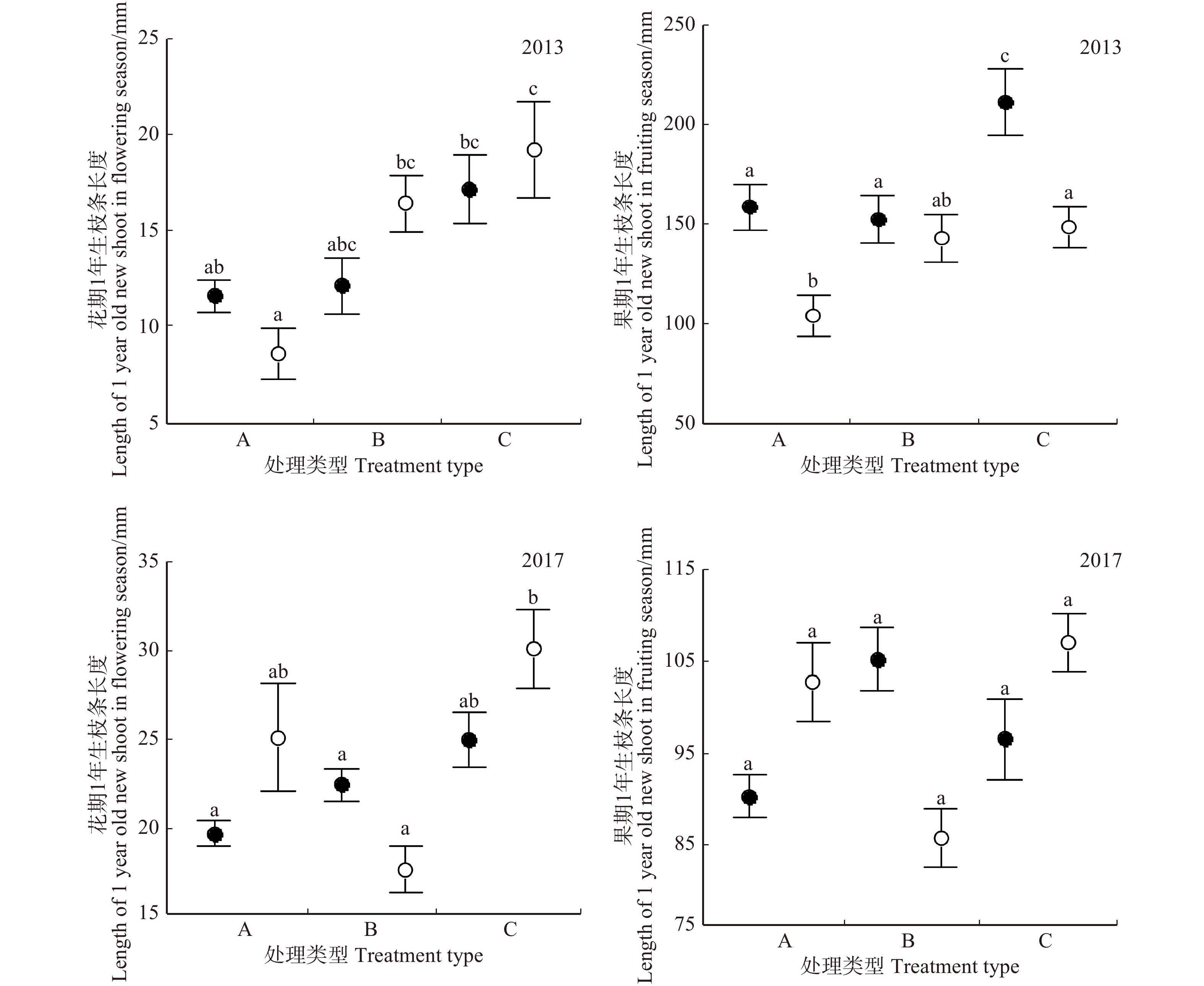
图 1 1年生枝条水平不同处理方式下簇毛槭1年生枝条长度对比

实心点为雌性，空心点为雄性。图中不同字母表示在P < 0.05水平上差异显著。下同。Solid point: female; hollow point: male. Varied letters denote significant differences at P < 0.05 level. Same as below.

Figure 1. Comparing the length of 1 year old new shoot under different treatments at shoot level for Acer barbinerve

下载: 全尺寸图片幻灯片

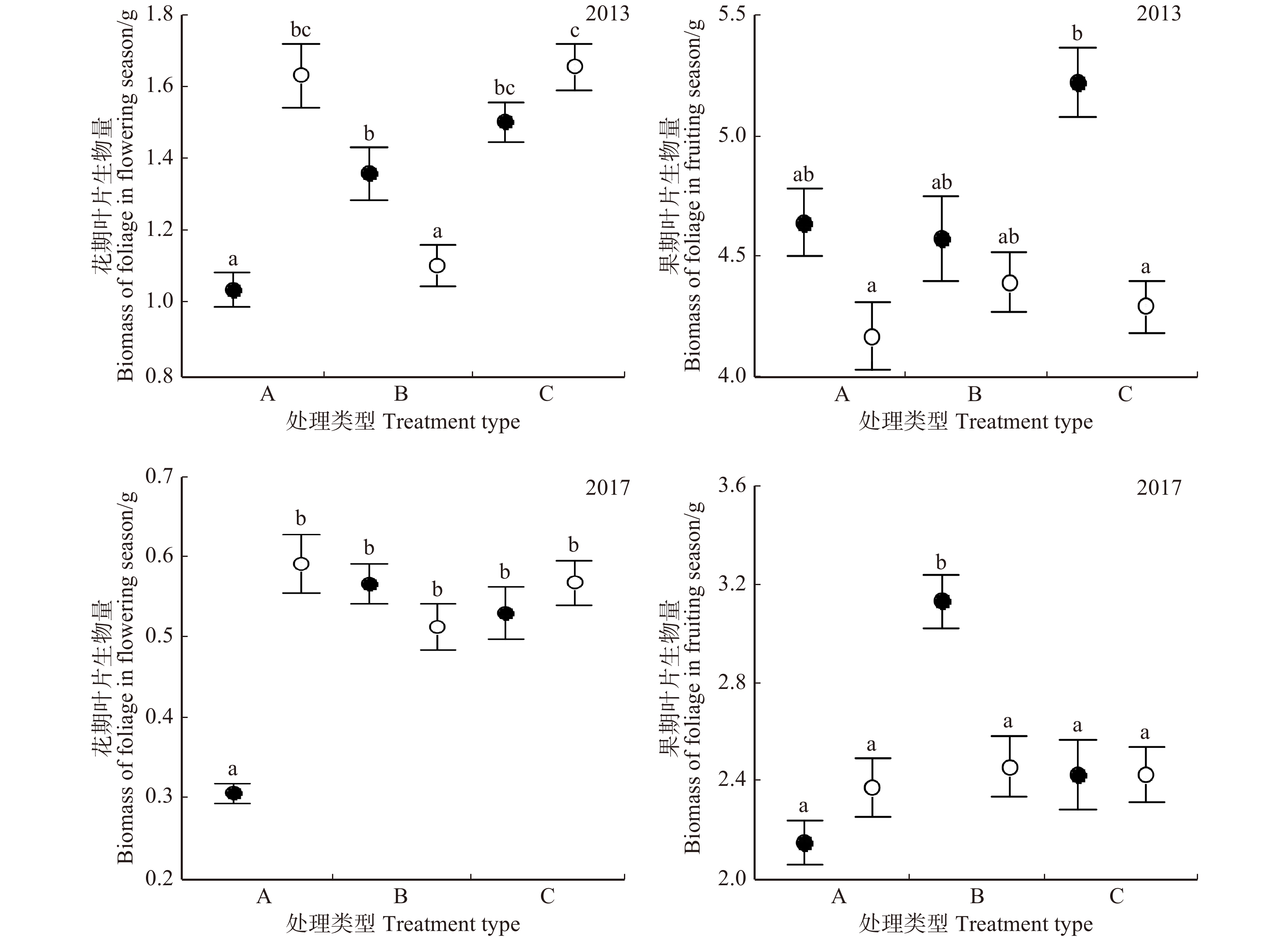
图 2 1年生枝条水平不同处理方式下簇毛槭叶片生物量对比

Figure 2. Comparing foliage biomass under different treatments at 1 year old new shoot level for Acer barbinerve

下载: 全尺寸图片幻灯片

图 3 2级侧枝水平不同处理方式下簇毛槭1年生枝条长度对比

实心点为雌性，空心点为雄性. 图中不同字母表示在P < 0.05水平上差异。Solid point: female; hollow point: male. Varied letters denote significant differences at P < 0.05 level.

Figure 3. Comparing the length of 1 year old new shoot under different treatments at grade 2 lateral branch level for Acer barbinerve

下载: 全尺寸图片幻灯片

图 4 2级侧枝水平不同处理方式下簇毛槭叶片生物量对比

Figure 4. Comparing foliage biomass under different treatments at grade 2 lateral branch level for Acer barbinerve

下载: 全尺寸图片幻灯片

表 1 试验选取的簇毛槭样株情况

Table 1 Sample individual conditions of Acer barbinerve

年份 Year	株数 Tree number	胸径 DBH/mm		树高 Tree height/m		冠幅东西 Crown diameter of east-west/m		冠幅南北 Crown diameter of north-south/m
年份 Year	株数 Tree number	雌株 Female	雄株 Male	雌株 Female	雄株 Male	雌株 Female	雄株 Male	雌株 Female	雄株 Male
2013	180	20.367a	19.176a	2.816a	2.543a	2.233a	2.051a	2.098a	2.085a
2017	145	21.511a	20.282a	2.720a	2.444a	2.553a	2.114b	2.224a	1.920a
注：不同字母表示在P < 0.05水平上差异显著。Note: different letters indicate significant difference at P < 0.05 level.

下载: 导出CSV

表 2 1年生枝条水平簇毛槭1年生枝条长度影响要素分析

Table 2 Analysis of influencing factors of the length of 1 year old new shoot at 1 year old shoot level for Acer barbinerve

变异来源 Variance source	2013年花期 Flowering season in 2013		2013年果期 Fruiting season in 2013		2017年花期 Flowering season in 2017		2017年果期 Fruiting season in 2017
变异来源 Variance source	F	P	F	P	F	P	F	P
性别 Gender	0.01	0.908	35.81	0.001	1.84	0.175	15.36	0.001
处理 Treatment	122.68	0.001	0.75	0.475	9.70	0.001	4.25	0.014
性别 × 处理 Gender × treatment	12.93	0.001	7.62	0.001	17.33	0.001	6.26	0.002

下载: 导出CSV

表 3 1年生枝条水平簇毛槭叶片生物量影响要素分析

Table 3 Influencing factors of biomass of foliage at 1 year old new shoot level for Acer barbinerve

变异来源 Variation source	2013年花期 Flowering season in 2013		2013年果期 Fruiting season in 2013		2017年花期 Flowering season in 2017		2017年果期 Fruiting season in 2017
变异来源 Variation source	F	P	F	P	F	P	F	P
性别 Gender	58.31	0.001	114.9	0.001	6.55	0.011	221.91	0.001
处理 Treatment	22.82	0.001	107.85	0.001	218.36	0.001	140.45	0.001
性别 × 处理 Gender × treatment	96.50	0.001	11.54	0.001	88.01	0.001	60.53	0.001

下载: 导出CSV

表 4 2级侧枝水平簇毛槭1年生枝条长度影响要素分析

Table 4 Influencing factors of the length of 1 year old new shoot at grade 2 lateral branch level for Acer barbinerve

变异来源 Variation source	2013年花期 Flowering season in 2013		2013年果期 Fruiting season in 2013		2017年花期 Flowering season in 2017		2017年果期 Fruiting season in 2017
变异来源 Variation source	F	P	F	P	F	P	F	P
性别 Gender	0.81	0.369	25.01	0.001	2.85	0.092	0.20	0.656
处理 Treatment	13.07	0.001	11.31	0.001	6.40	0.002	0.68	0.507
性别 × 处理 Gender × treatment	2.85	0.058	3.35	0.036	4.39	0.013	5.04	0.007

下载: 导出CSV

表 5 2级侧枝水平簇毛槭叶片生物量影响要素分析

Table 5 Influencing factors of the biomass of foliage at grade 2 lateral branch level for Acer barbinerve

变异来源 Variation source	2013年花期 Flowering season in 2013		2013年果期 Fruiting season in 2013		2017年花期 Flowering season in 2017		2017年果期 Fruiting season in 2017
变异来源 Variation source	F	P	F	P	F	P	F	P
性别 Gender	15.50	0.001	11.85	0.001	22.31	0.001	3.35	0.068
处理 Treatment	19.14	0.001	1.94	0.145	17.95	0.001	16.60	0.001
性别 × 处理 Gender × treatment	23.27	0.001	1.88	0.153	21.93	0.001	7.86	0.001

下载: 导出CSV

参考文献(49)

[1]	Karlsson P S, Andersson M, Svensson B M. Relationships between fruit production and branching in monocarpic shoot modules of Rhododendron lapponicum[J]. Ecoscience, 2006, 13(3): 396−403. doi: 10.2980/i1195-6860-13-3-396.1
[2]	Berger J D, Shrestha D, Ludwig C. Reproductive strategies in Mediterranean Legumes: trade-offs between phenology, seed size and vigor within and between wild and domesticated Lupinus Species collected along aridity gradients [J/OL]. Frontiers in Plant Science, 2017, (2017−04−13)[2018−01−20]. https://doi.org/10.3389/fpls.2017.00548.
[3]	Obeso J R. Costs of reproduction in Ilex aquifolium: effects at tree, branch and leaf levels[J]. Journal of Ecology, 1997, 85(2): 159−166. doi: 10.2307/2960648
[4]	Nicotra A B. Reproductive allocation and the long-term costs of reproduction in Siparuna grandiflora, a dioecious neo-tropical shrub[J]. Journal of Ecology, 1999, 87(1): 138−149. doi: 10.1046/j.1365-2745.1999.00337.x
[5]	Miyazaki Y. Dynamics of internal carbon resources during masting behavior in trees[J]. Ecological Research, 2013, 28(2): 143−150. doi: 10.1007/s11284-011-0892-6
[6]	Thorén L M, Karlsson P S, Tuomi J. Somatic cost of reproduction in three carnivorous Pinguicula species[J]. Oikos, 1996, 76(3): 427−434. doi: 10.2307/3546336
[7]	Newell E A. Direct and delayed costs of reproduction in Aesculus californica[J]. Journal of Ecology, 1991, 79(2): 365−378. doi: 10.2307/2260719
[8]	Ehrlén J, Van Groenendael J. Storage and the delayed costs of reproduction in the understorey perennial Lathyrus vernus[J]. Journal of Ecology, 2001, 89(2): 237−246. doi: 10.1046/j.1365-2745.2001.00546.x
[9]	Horvitz C C, Schemske D W. Demographic cost of reproduction in a neotropical herb: an experimental field study[J]. Ecology, 1988, 69(6): 1741−1745. doi: 10.2307/1941152
[10]	Horibata S, Hasegawa S F, Kudo G. Cost of reproduction in a spring ephemeral species, Adonis ramosa (Ranunculaceae): carbon budget for seed production[J]. Annals of Botany, 2007, 100(3): 565−571. doi: 10.1093/aob/mcm131
[11]	Matsuyama S, Sakimoto M. Sexual dimorphism of reproductive allocation at shoot and tree levels in Zanthoxylum ailanthoides, a pioneer dioecious tree[J]. Botanique, 2010, 88(10): 867−874. doi: 10.1139/B10-058
[12]	Cipollini M L, Whigham D F. Sexual dimorphism and cost of reproduction in the dioecious shrub Lindera benzoin (Lauraceae)[J]. American Journal of Botany, 1994, 81(1): 65−75. doi: 10.1002/j.1537-2197.1994.tb15410.x
[13]	Bañuelos M J, Obeso J R. Resource allocation in the dioecious shrub Rhamnus alpinus: the hidden costs of reproduction[J]. Evolutionary Ecology Research, 2004, 6(3): 397−413.
[14]	Mge M, Antos J A, Allen G A. Modules of reproduction in females of the dioecious shrub Oemleria cerasiformis[J]. Revue Canadienne De Botanique, 2004, 82(3): 393−400.
[15]	Matsuyama S, Sakimoto M. Allocation to reproduction and relative reproductive costs in two species of dioecious Anacardiaceae with contrasting phenology[J]. Annals of Botany, 2008, 101(9): 1391−1400. doi: 10.1093/aob/mcn048
[16]	Geber M A, Dawson T E, Delph L F. Gender and sexual dimorphism in flowering plants [M]. Berlin: Springer, 1999: 33−60.
[17]	Delph L F, Knapczyk F N, Taylor D R. Among-population variation and correlations in sexually dimorphic traits of Silene latifolia[J]. Journal of Evolutionary Biology, 2010, 15(6): 1011−1020.
[18]	Chen J, Niu Y, Yang Y, et al. Sexual allocation in the gynodioecious species Cyananthus macrocalyx (Campanulaceae) at high elevations in the Sino-Himalaya Mountains[J]. Alpine Botany, 2016, 126(1): 49−57. doi: 10.1007/s00035-015-0154-2
[19]	Huan H, Wang B, Liu G, et al. Sexual differences in morphology and aboveground biomass allocation in relation to branch number in Morus alba saplings[J]. Australian Journal of Botany, 2016, 64(3): 269−275. doi: 10.1071/BT15189
[20]	Fonseca D C, Oliveira M L R, Pereira I M, et al. Phenological strategies of dioecious species in response to the environmental variations of rupestrian grasslands[J]. Cerne, 2018, 23(4): 517−527.
[21]	Juvany M, Munnébosch S. Sex-related differences in stress tolerance in dioecious plants: a critical appraisal in a physiological context[J]. Journal of Experimental Botany, 2015, 66(20): 6083−6092. doi: 10.1093/jxb/erv343
[22]	Chen J, Duan B, Wang M, et al. Intra-and inter-sexual competition of Populus cathayana under different watering regimes[J]. Functional Ecology, 2014, 28(1): 124−136. doi: 10.1111/fec.2014.28.issue-1
[23]	Wang J, Zhang C, Zhao X, et al. Reproductive allocation of two dioecious Rhamnus species in temperate forests of northeast China[J]. Iforest Biogeosciences & Forestry, 2013, 7(1): 25−32.
[24]	Zang R G, Xu H C. Canopy disturbance regimes and gap regeneration in a Korena pine-broadleaved forest in Jiaohe, northeast China[J]. Bulletin of Botanical Research, 1999, 19(2): 112−120.
[25]	中国科学院中国植物志委员会. 中国植物志: 1卷[M]. 北京: 科学出版社, 2004. The Chinese Flora of the Chinese Academy of Sciences. Flora of China: I [M]. Beijing: Science Press, 2004.
[26]	Zajitschek F, Connallon T. Partitioning of resources: the evolutionary genetics of sexual conflict over resource acquisition and allocation[J]. Journal of Evolutionary Biology, 2017, 30(4): 826−838. doi: 10.1111/jeb.2017.30.issue-4
[27]	Tonnabel J, David P, Pannell J R. Sex-specific strategies of resource allocation in response to competition for light in a dioecious plant[J]. Oecologia, 2017, 185(4): 675−686. doi: 10.1007/s00442-017-3966-5
[28]	Sletvold N J Å. Climate-dependent costs of reproduction: survival and fecundity costs decline with length of the growing season and summer temperature[J]. Ecology Letters, 2015, 18(4): 357−364. doi: 10.1111/ele.2015.18.issue-4
[29]	Hossain S M Y, Caspersen J P, Thomas S C. Reproductive costs in Acer saccharum: exploring size-dependent relations between seed production and branch extension[J]. Trees, 2017, 31(4): 1−10.
[30]	Xiao Y A, Dong M, Wang N, et al. Effects of organ removal on trade-offs between sexual and clonal reproduction in the stoloniferous herb Duchesnea indica[J]. Plant Species Biology, 2016, 31(1): 50−54. doi: 10.1111/psbi.2016.31.issue-1
[31]	Torimaru T, Tomaru N. Reproductive investment at stem and genet levels in male and female plants of the clonal dioecious shrub Ilex leucoclada (Aquifoliaceae)[J]. Botanique, 2012, 90(4): 301−310. doi: 10.1139/b2012-004
[32]	Teitel Z, Pickup M, Field D L, et al. The dynamics of resource allocation and costs of reproduction in a sexually dimorphic, wind-pollinated dioecious plant[J]. Plant Biology, 2016, 18(1): 98−103. doi: 10.1111/plb.12336
[33]	Leigh A, Cosgrove M, Nicotra A. Reproductive allocation in a gender dimorphic shrub: anomalous female investment in Gynatrix pulchella[J]. Journal of Ecology, 2006, 94(6): 1261−1271. doi: 10.1111/jec.2006.94.issue-6
[34]	Hasegawa S, Takeda H. Functional specialization of current shoots as a reproductive strategy in Japanese alder (Alnus hirsuta var.sibirica)[J]. Canadian Journal of Botany, 2001, 79(1): 38−48.
[35]	Díaz-Barradas M C, Zunzunegui M, Collantes M, et al. Gender-related traits in the dioecious shrub Empetrum rubrum in two plant communities in the Magellanic steppe[J]. Acta Oecologica, 2014, 60(10): 40−48.
[36]	Xiao Y, Zhao H, Yang W, et al. Variations in growth, clonal and sexual reproduction of Spartina alterniflora responding to changes in clonal integration and sand burial[J]. CLEAN − Soil, Air, Water, 2015, 43(7): 1100−1106. doi: 10.1002/clen.v43.7
[37]	Wang H, Matsushita M, Tomaru N, et al. Differences in female reproductive success between female and hermaphrodite individuals in the subdioecious shrub Eurya japonica (Theaceae)[J]. Plant Biology, 2015, 17(1): 194−200. doi: 10.1111/plb.12189
[38]	Midgley J J. Causes of secondary sexual differences in plants : evidence from extreme leaf dimorphism in Leucadendron (Proteaceae)[J]. South African Journal of Botany, 2010, 76(3): 588−592. doi: 10.1016/j.sajb.2010.05.001
[39]	Jaquish L L, Ewers F W. Seasonal conductivity and embolism in the roots and stems of two clonal ring: porous trees, Sassafras albidum (Lauraceae) and Rhus typhina (Anacardiaceae)[J]. American Journal of Botany, 2001, 88(2): 206−212. doi: 10.2307/2657011
[40]	Zunzunegui M, Barradas M C D, Clavijo A, et al. Ecophysiology, growth timing and reproductive effort of three sexual foms of Corema album (Empetraceae)[J]. Plant Ecology, 2006, 183(1): 35−46. doi: 10.1007/s11258-005-9004-4
[41]	Milla R, Castrodíez P, Maestromartínez M, et al. Costs of reproduction as related to the timing of phenological phases in the dioecious shrub Pistacia lentiscus L.[J]. Plant Biology, 2006, 8(1): 103−111. doi: 10.1055/s-2005-872890
[42]	Nicotra A B. Sexually dimorphic growth in the dioecious tropical shrub, Siparuna grandiflora[J]. Functional Ecology, 2010, 13(3): 322−331.
[43]	Sánchez V J, Pannell J R. Sexual dimorphism in resource acquisition and deployment: both size and timing matter[J]. Annals of Botany, 2011, 107(1): 119−126. doi: 10.1093/aob/mcq209
[44]	Tozawa M, Ueno N, Seiwa K. Compensatory mechanisms for reproductive costs in the dioecious tree Salix integra[J]. Botany-botanique, 2009, 87(3): 315−323. doi: 10.1139/B08-125
[45]	Álvarez-Cansino L, Zunzunegui M, Barradas M C D, et al. Gender-specific costs of reproduction on vegetative growth and physiological performance in the dioecious shrub Corema album[J]. Annals of Botany, 2010, 106(6):989−998.
[46]	Fujii S, Toriyama K. Suppressed expression of retrogrand - regulated male sterility restores pollen fertility in cytoplasmic male sterile rice plants[J]. Proceedings of the National Academy of Sciences of the United States of America, 2009, 106(23): 9513−9518. doi: 10.1073/pnas.0901860106
[47]	Kumar N, Gupta S, Tripathi A N. Gender-specific responses of Piper betle L. to low temperature stress: changes in chlorophyllase activity[J]. Biologia Plantarum, 2006, 50(4): 705−708. doi: 10.1007/s10535-006-0111-4
[48]	Aschan G, Pfanz H. Non-foliar photosynthesis: a strategy of additional carbon acquisition[J]. Flora, 2003, 198(2): 81−97. doi: 10.1078/0367-2530-00080
[49]	Cai Z Q. Shade delayed flowering and decreased photosynthesis, growth and yield of Sacha Inchi (Plukenetia volubilis) plants[J]. Industrial Crops & Products, 2011, 34(1): 1235−1237.

施引文献(20)

期刊类型引用(9)

1.	辛守英，王晓红，焦琳琳. 基于遥感数据和优化Blending算法的人工林地上生物量估算研究. 西北林学院学报. 2025(02): 207-219 . 百度学术
2.	郝君，吕康婷，胡天祺，王云阁，徐刚. 基于机器学习的红树林生物量遥感反演研究. 林草资源研究. 2024(01): 65-72 . 百度学术
3.	李敏，陈利，李静泰，闫丹丹，刘垚，吴翠玲，栾兆擎. 基于Sentinel-2数据的互花米草地上生物量反演. 海洋环境科学. 2024(03): 386-397 . 百度学术
4.	廖易，张加龙，鲍瑞，许冬凡. 基于Landsat的高山松地上生物量动态变化估测模型构建. 西南林业大学学报(自然科学). 2023(01): 117-125 . 百度学术
5.	郭芮，伏帅，侯蒙京，刘洁，苗春丽，孟新月，冯琦胜，贺金生，钱大文，梁天刚. 基于Sentinel-2数据的青海门源县天然草地生物量遥感反演研究. 草业学报. 2023(04): 15-29 . 百度学术
6.	廖易，张加龙，鲍瑞，许冬凡，王书贤，韩冬阳. 引入地形因子的高山松地上生物量动态估测. 生态学杂志. 2023(05): 1243-1252 . 百度学术
7.	王熙媛，张王菲，李云，杨仙保. 依据光学遥感特征优选的森林地上生物量反演. 东北林业大学学报. 2022(04): 47-54 . 百度学术
8.	陈园园，张晓丽，高显连，高金萍. 基于Sentinel-1和Sentinel-2A的西小山林场平均树高估测. 应用生态学报. 2021(08): 2839-2846 . 百度学术
9.	陈小芳，李军，李新伟，周毅. 基于高光谱的水稻生物量估测模型研究. 安徽科技学院学报. 2021(05): 53-59 . 百度学术

其他类型引用(11)

资源附件(0)

图(4) / 表(5)

计量

文章访问数: 2486
HTML全文浏览量: 890
PDF下载量: 71
被引次数: 20

1. 研究区概况
2. 研究方法
2.1 地面数据采集与生物量计算
2.2 Sentinel-2A数据
2.3 数字高程模型DEM数据
2.4 分类辅助数据
2.5 变量提取
2.6 生物量估算模型的建立与评价
3. 结果与分析
3.1 Sentinel-2A数据与生物量的关系
3.2 生物量预测及评价
4. 讨　　论
5. 结　　论

1. 研究区概况
2. 研究方法
2.1 地面数据采集与生物量计算
2.2 Sentinel-2A数据
2.3 数字高程模型DEM数据
2.4 分类辅助数据
2.5 变量提取
2.6 生物量估算模型的建立与评价
3. 结果与分析
3.1 Sentinel-2A数据与生物量的关系
3.2 生物量预测及评价
4. 讨　　论
5. 结　　论

参考文献(49)

施引文献(20)

资源附件(0)

雌雄异株植物簇毛槭繁殖代价延迟效应研究

作者简介: 赵海艳。主要研究方向：繁殖生态学。Email：zhaohaiyan_2016@163.com 地址：100083北京市海淀区清华东路35号北京林业大学林学院

责任作者: 王娟，副教授。主要研究方向：繁殖生态学。Email：wangjuan@bjfu.edu.cn 地址：同上

计量

出版历程